Where a Weight Lives, in JAX/Flax NNX

The explainer argued that a standard weight is a direction in a space apart from the data, and that a reproducing kernel Hilbert space repairs that by giving the weight an address among the data: the optimal weight is a combination of the data’s own kernel bumps. This is the implementation. A kernel in a few lines of JAX, the Gram matrix, one linear solve for the coefficients, and the weight comes out as $\sum_i \alpha_i\, k(x_i, \cdot)$. Then two demonstrations of why the shared space matters. Every number is from a real run; the script is scripts/render_weight_lives_gifs.py.

Prefer a notebook? Run the whole thing on Kaggle: the same code, block by block, with the math written out and every figure reproduced from a real run.

The kernel, and the space it builds#

Where does the shared space come from? One function: a reproducing kernel is any positive-definite similarity, and the whole RKHS hangs off it. We use the radial basis kernel, a bump that is largest when two points coincide and decays with their distance. In JAX it is one expression, and it gives the inner product $\langle \phi(x), \phi(y)\rangle$ without ever forming $\phi$.

import jax, jax.numpy as jnp

SIG = 0.5

@jax.jit
def gram(X, Y):                                        # k(xᵢ, yⱼ) for every pair
    d2 = ((X[:, None, :] - Y[None, :, :]) ** 2).sum(-1)
    return jnp.exp(-d2 / (2 * SIG ** 2))

That gram(X, X) is the entire geometry of the data in the RKHS: entry (i, j) is how close points i and j sit once lifted by φ. Nothing about the weight yet, only the space the weight will live in.

The weight is a solve, not a search#

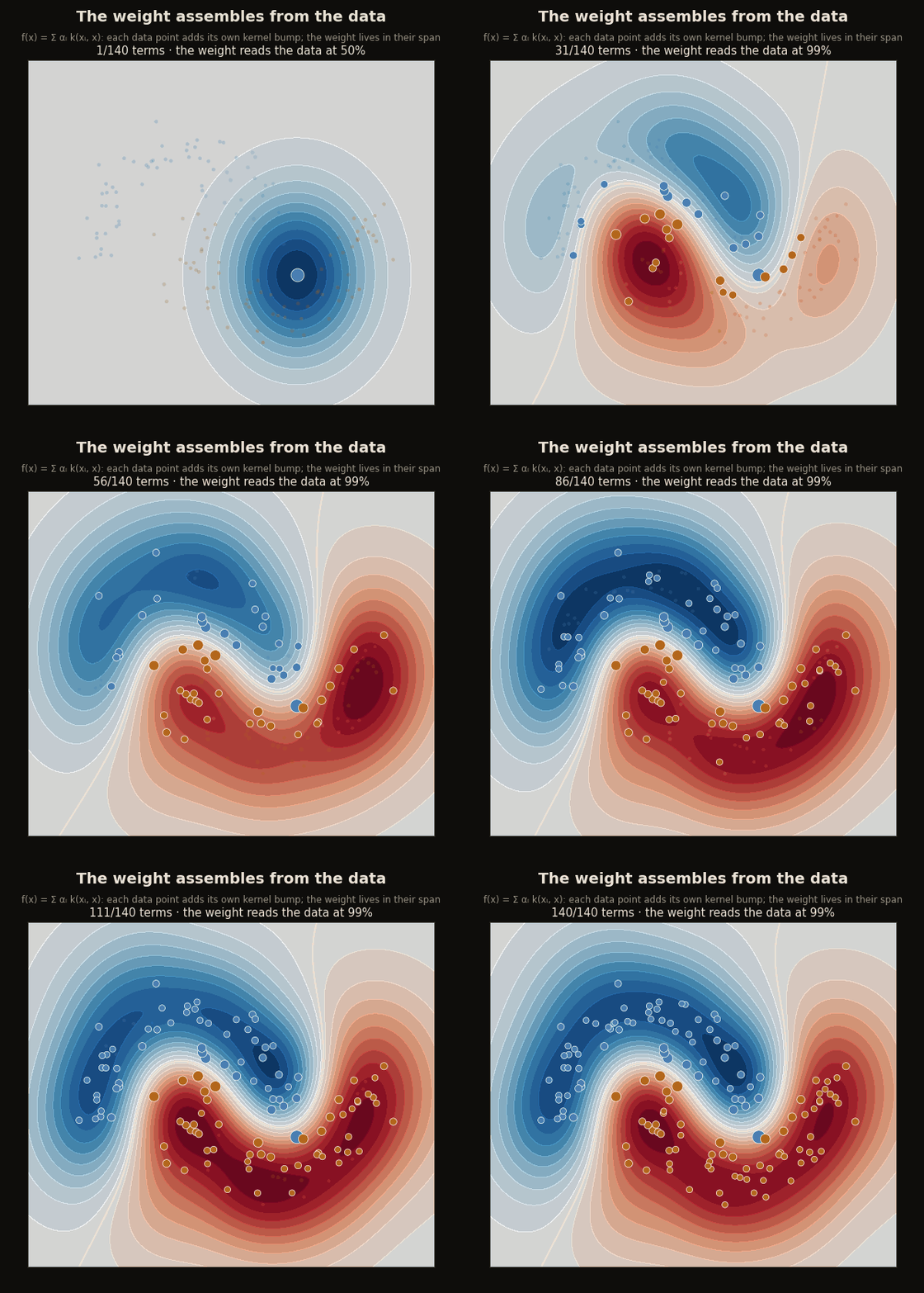
So where is the weight in all this? The representer theorem promises the optimal one is $f(x) = \sum_i \alpha_i\, k(x_i, x)$, a combination of the data. Fitting the weight is therefore not a gradient descent through some separate weight space; it is solving for the coefficients $\alpha_i$ that make the combination match the labels. With a ridge penalty that is a single linear system, $(G + \lambda I)\,\alpha = y$.

def kernel_ridge(X, y, lam=0.4):                       # the representer coefficients
    G = gram(X, X)
    return jnp.linalg.solve(G + lam * jnp.eye(len(X)), y)

The vector alpha that comes back is the weight, expressed in the only basis the RKHS gives you for free: the data points themselves. Each $\alpha_i$ is the charge on point $x_i$. To evaluate the weight anywhere you weigh the kernels by $\alpha$, which is gram(grid, X) @ alpha. Watch it assemble: the heaviest coefficients first, each adding its own bump, the decision boundary forming out of the data.

Why the shared space is worth it#

The explainer closed on the claim that a placed weight can bend around nested classes where any direction sits at chance; here is that claim as two numbers. The best linear weight is found by scikit-learn’s logistic regression (the one non-JAX import in this post; everything kernel is plain JAX), and it lands at a coin flip, because no direction separates an inner disk from an outer ring. The kernel weight, the same α solve, wraps a closed boundary around the inner ring.

from sklearn.datasets import make_circles
from sklearn.linear_model import LogisticRegression

X, y = make_circles(260, noise=0.07, factor=0.4, random_state=0)
ys = jnp.where(jnp.asarray(y) == 1, 1.0, -1.0)

lin = LogisticRegression().fit(X, y)                   # a direction
alpha = kernel_ridge(jnp.asarray(X), ys, lam=0.2)      # a placed combination
k_pred = jnp.sign(gram(jnp.asarray(X), jnp.asarray(X)) @ alpha)
print(f"line: {100*lin.score(X, y):.0f}%   kernel: {100*(k_pred == ys).mean():.0f}%")
# line: 50%   kernel: 100%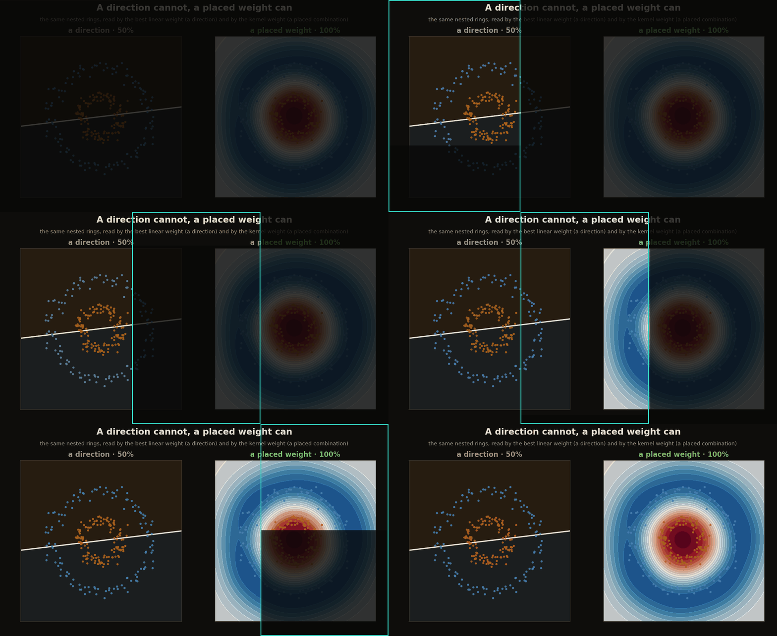

How the placed weight reads a point#

Notice what the rings demo never did: it never built a single new coordinate. There is no explicit feature vector anywhere in this code, no lifted space we construct by hand. The prediction at a query is the reproducing property made literal, $f(q) = \langle f, \phi(q)\rangle = \sum_i \alpha_i\, k(x_i, q)$: the query is compared to each data point by the kernel, those similarities are scaled by the coefficients, and the signed sum is the score. The feature map $\phi$ exists in the theory, but the code only ever touches it through $k$.

q = jnp.array([1.7, -0.35])
kq = jnp.exp(-((jnp.asarray(X) - q) ** 2).sum(1) / (2 * SIG ** 2))   # k(xᵢ, q)
fq = (alpha * kq).sum()                                             # f(q) = Σ αᵢ k(xᵢ, q)
print(f"f(q) = {fq:+.2f}  ->  {'orange' if fq >= 0 else 'blue'} class")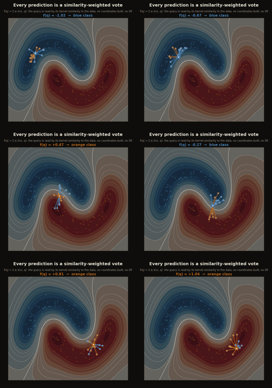

The weight never left the data. It is a list of coefficients on the points you already have, solved in one shot, read by similarity. That is the whole of what it means to have a reproducing kernel Hilbert space: the weight and the data finally share a space, and the weight is just the data, recombined.

The RKHS is Aronszajn (1950); the representer theorem is Schölkopf, Herbrich and Smola (2001); the textbook is Schölkopf and Smola (2002); the input-space-center kernel is Bouhsine (2026). The conceptual companion is Where Does a Weight Live?.

@misc{bouhsine2026wheredoesaweightlivejaxflaxnnx,
  author       = {Bouhsine, Taha},
  title        = {Where a Weight Lives, in JAX/Flax NNX},
  year         = {2026},
  month        = {jun},
  howpublished = {\url{https://tahabouhsine.com/blog/where-does-a-weight-live-jax-flax-nnx/}},
  note         = {Blog post, Records of the !mmortal Data Scientist}
}