Calibrating a Bounded Net, in JAX/Flax NNX

The explainer put a bounded kernel MLP’s confidence on trial against a matched ReLU MLP and found, against the series’ own bet, that the interpretable network is the one whose probabilities lie. This is the implementation: build both nets in Flax NNX with the exact same softmax head, then measure their honesty with reliability diagrams, ECE, temperature scaling, and the two out-of-distribution channels. Every number below is from a real three-seed run; the script is scripts/yat_calibration.py.

Prefer a notebook? Run the whole thing on Kaggle: the same code, block by block, with the math written out and every figure reproduced from a real run.

Two nets, one head#

What makes a calibration test fair? That confidence means the same thing for both contestants. So the two networks share everything downstream of the feature map: a linear readout to ten logits, then a softmax, then the max. Only the layer that turns an image into features differs, and that is the whole experiment. The Yat layer scores each input against K prototypes with the kernel from the earlier posts; the ReLU layer is the ordinary affine-then-rectify.

import jax, jax.numpy as jnp
from flax import nnx

K = 50

class YatLayer(nnx.Module):
    """Each unit is the Yat kernel against a prototype row of W."""
    def __init__(self, *, rngs, Winit, b0=1.0, eps0=1.0):
        self.W = nnx.Param(jnp.asarray(Winit))                       # [K, 784] prototypes
        self.log_b = nnx.Param(jnp.full((), jnp.log(jnp.expm1(b0))))
        self.log_eps = nnx.Param(jnp.full((), jnp.log(jnp.expm1(eps0))))

    def __call__(self, x):
        b = jax.nn.softplus(self.log_b.value)
        eps = jax.nn.softplus(self.log_eps.value)
        dot = x @ self.W.value.T
        d2 = jnp.sum(x ** 2, -1, keepdims=True) + jnp.sum(self.W.value ** 2, -1) - 2 * dot
        return (dot + b) ** 2 / (d2 + eps)                           # [N, K] kernel scores

class YatMLP(nnx.Module):
    def __init__(self, *, rngs, Winit):
        self.yat = YatLayer(rngs=rngs, Winit=Winit)
        self.readout = nnx.Linear(K, 10, rngs=rngs)
    def __call__(self, x):
        return self.readout(self.yat(x))                            # logits

class ReluMLP(nnx.Module):
    def __init__(self, *, rngs):
        self.l1 = nnx.Linear(784, K, rngs=rngs)
        self.l2 = nnx.Linear(K, 10, rngs=rngs)
    def __call__(self, x):
        return self.l2(jax.nn.relu(self.l1(x)))                     # logits

Both are one hidden layer of 50 units, 784 -> 50 -> 10. The Yat net’s prototypes are seeded from training images, the ReLU net is the same shape, and both train with plain cross-entropy. That last detail matters for the story: nothing in the objective ever asks the confidence to be honest, only correct.

import optax

@nnx.jit
def train_step(model, opt, xb, yb):
    def loss_fn(m):
        return optax.softmax_cross_entropy_with_integer_labels(m(xb), yb).mean()
    loss, grads = nnx.value_and_grad(loss_fn)(model)
    opt.update(model, grads)
    return loss

The data split is fixed once and reused for both nets: 55,000 Fashion-MNIST images to train on, 5,000 held out for temperature scaling only, the full 10,000 test set for the diagrams, and MNIST’s test digits as the out-of-distribution probe. We train each net on three seeds (0, 1, 2) so every verdict below carries an error bar.

The forecaster’s test, in code#

How do you catch a network overstating its confidence? Bin its predictions by claimed confidence and, in each bin, compare the claim against the accuracy it actually delivered. That comparison is the reliability diagram, and averaging its per-bin gaps, weighted by how many predictions live in each bin, is the expected calibration error. Confidence is read identically from both nets: softmax the logits, take the max.

import numpy as np

def softmax(z):
    z = z - z.max(1, keepdims=True); e = np.exp(z)
    return e / e.sum(1, keepdims=True)

def reliability(z, y, n_bins=15):
    p = softmax(z); conf = p.max(1); pred = p.argmax(1)
    correct = (pred == y).astype(float)
    edges = np.linspace(0, 1, n_bins + 1)
    idx = np.clip(np.digitize(conf, edges[1:-1]), 0, n_bins - 1)
    count = np.zeros(n_bins); mconf = np.zeros(n_bins); macc = np.zeros(n_bins)
    for b in range(n_bins):
        m = idx == b
        count[b] = m.sum()
        if count[b] > 0:
            mconf[b] = conf[m].mean(); macc[b] = correct[m].mean()
    ece = float((count / len(y) * np.abs(macc - mconf)).sum())      # count-weighted |acc - conf|
    return count, mconf, macc, ece

Run it on both nets and the staircases part ways. The ReLU bars land on the diagonal; the Yat bars sag below it, claiming more than they deliver in almost every bin.

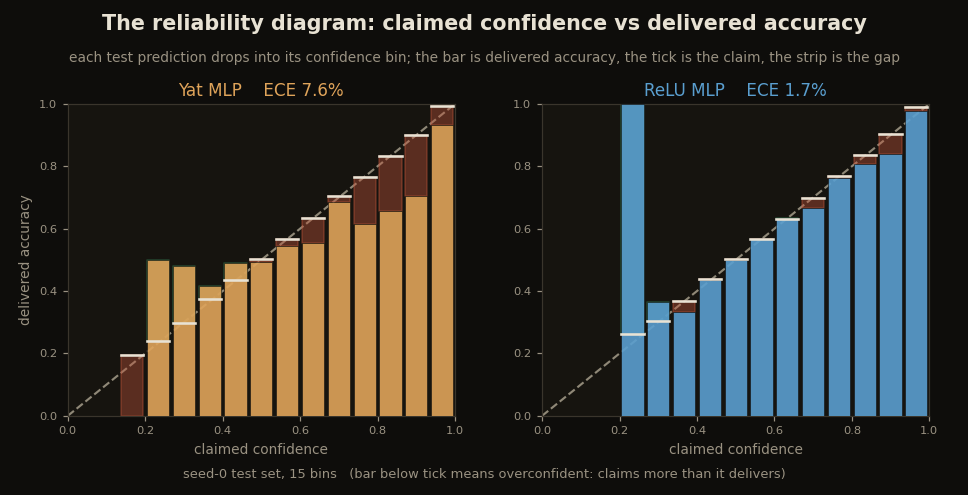
Averaged over the three seeds the numbers are stark. The ReLU net’s ECE is 1.76% ± 0.22; the Yat net’s is 6.20% ± 1.13, between three and four times worse. The proper scoring rules agree: NLL 0.360 vs 0.577, Brier 0.181 vs 0.244.

def nll_of(z, y):
    p = softmax(z)
    return float(-np.log(np.clip(p[np.arange(len(y)), y], 1e-12, 1)).mean())

def brier_of(z, y):
    p = softmax(z); onehot = np.eye(10)[y]
    return float(((p - onehot) ** 2).sum(1).mean())

Why the bounded net brags#

Where does the overconfidence come from? Not from the objective, and not from a bug: from the units. A Yat unit is a kernel score, and near its prototype that score is large, with a median strongest match around 207 on the seed-0 test set. The linear readout inherits that dynamic range, so the median top logit of the Yat net is 28.9 against the ReLU net’s 7.2. And the softmax does not read logits, it reads gaps between them, exponentiated. A lead of a few units already pins the winner near probability one.

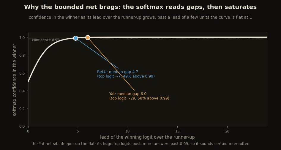
So the fix should be a unit conversion. That is temperature scaling.

One knob, fit on held-out data#

Temperature scaling divides every logit by a single scalar T before the softmax, and picks T on the held-out split by minimizing NLL. It never touches the argmax, so accuracy is untouched; it only changes how loudly the network states what it already decided.

from scipy.optimize import minimize_scalar

def fit_temperature(z_val, y_val):
    def obj(logT):                                                  # search in log-space, T > 0
        return nll_of(z_val / np.exp(logT), y_val)
    r = minimize_scalar(obj, bounds=(np.log(0.05), np.log(20.0)), method='bounded')
    return float(np.exp(r.x))

Turn the knob and the Yat reliability curve rotates toward the diagonal as its held-out loss draws down to its minimum. That minimum lands at T = 2.07 on seed 0, meaning the raw net was more than twice as loud as it should have been.

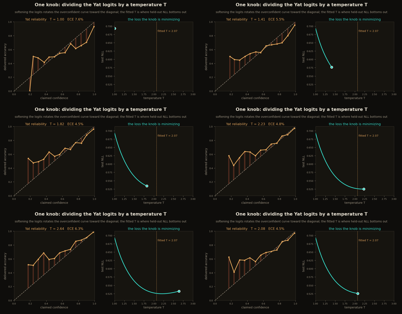
Does the prototype net at least need less correction? The opposite. The ReLU net’s fitted temperature is 1.17 ± 0.02, a nudge; the Yat net needs 1.68 ± 0.29, and its temperature swings from 1.37 to 2.07 across the three seeds while the ReLU net’s barely moves. Worse, one knob cannot close the gap, because the Yat curve is bent rather than merely tilted: after scaling the ReLU net sits at ECE 0.82% and the Yat net at 3.11%, still three to four times worse. Calibration lives in the head, and both nets have the same head. The kernel just feeds it wilder numbers.

The number the softmax throws away#

That is the in-distribution verdict, and it goes to the black box. But the earlier posts made their “knows when it doesn’t know” claim off-distribution, so feed both nets MNIST digits, handwriting shown to a garment classifier, and read the confidence differently. Softmax has a blind spot: add a constant to every logit and it does not move, so it is a contrast reader that cannot see the absolute level. And absolute level is exactly how a bounded kernel says “I recognize nothing here”: off-distribution every well is shallow and all ten scores sink together. So ask the same forward pass two questions, one before the softmax and one after.

# the pre-softmax field magnitude: the strongest kernel match, straight off the Yat layer
kmax_test = np.asarray(yat.yat(jnp.asarray(Xte))).max(1)            # [N_test]
kmax_ood  = np.asarray(yat.yat(jnp.asarray(Xood))).max(1)           # [N_ood]

# the same forward pass, read after the softmax
conf_test = softmax(logits_of(yat, Xte)).max(1)
conf_ood  = softmax(logits_of(yat, Xood)).max(1)

def auroc(pos, neg):                                                # rank-based, ties averaged
    s = np.concatenate([pos, neg]); order = np.argsort(s, kind='mergesort')
    ranks = np.empty(len(s)); sr = s[order]; i = 0
    while i < len(sr):
        j = i
        while j + 1 < len(sr) and sr[j + 1] == sr[i]: j += 1
        ranks[order[i:j + 1]] = 0.5 * (i + j) + 1; i = j + 1
    rp = ranks[:len(pos)].sum()
    return float((rp - len(pos) * (len(pos) + 1) / 2) / (len(pos) * len(neg)))

Read before the softmax, the two datasets pull apart; read after it, they smear together.

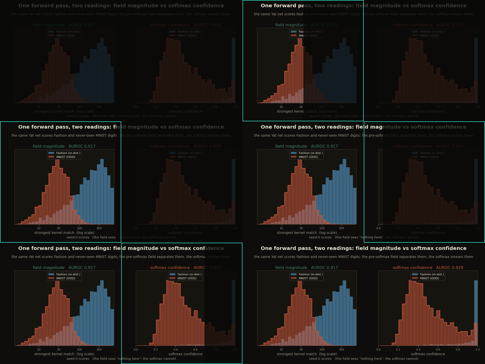
Across the three seeds the field magnitude separates Fashion from MNIST at AUROC 0.916 ± 0.008. The comparison the literature demands is the ReLU net’s max logit, the well-known max-logit and energy score, which reaches 0.935 ± 0.005, a touch better; magnitude as an OOD signal is not the kernel’s invention. What the field wins is not the third decimal, it is stability and meaning: a kernel score of 27 against a typical 207 is a sentence you can say out loud before running any benchmark, and it holds through every retraining.

The channel that does not wobble#

Which is the last thing to see, because it is the whole reason to route the OOD question around the softmax. Retrain the net three times and recompute both channels, and the softmax channel’s separation lurches from seed to seed while the field channel holds.

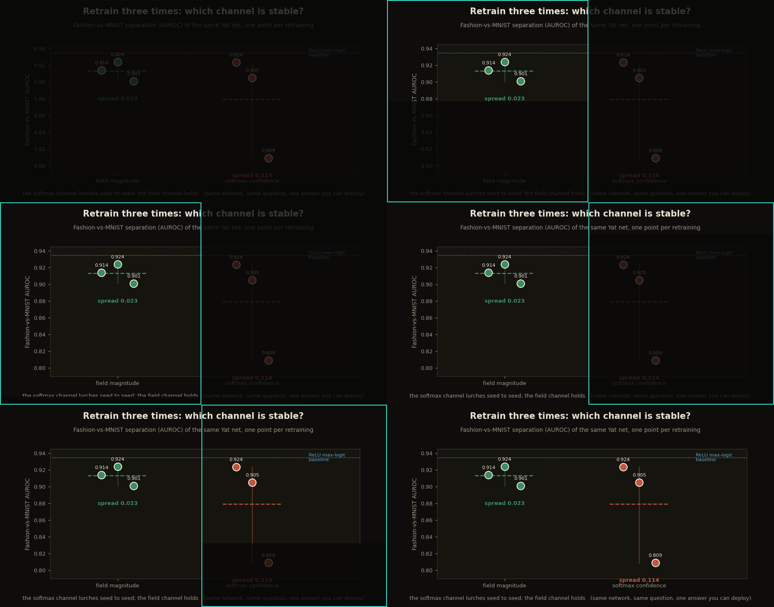
The field magnitude reads AUROC 0.914, 0.924, 0.901 across the seeds; the softmax reads 0.924, 0.905, 0.809. On a bad retraining the softmax channel is barely better than the ReLU baseline, while the field never has the bad day. That is the abstention rule from the earlier posts, now with its error bars measured.

What the experiment settled#

The scoreboard, all three seeds. In-distribution the ReLU net wins outright: ECE 1.76% against 6.20%, temperature 1.17 against 1.68, and it stays ahead after both are corrected, because the kernel’s dynamic range saturates the softmax. Off-distribution the field magnitude, the number the softmax deletes, separates Fashion from MNIST at a steady 0.92 while the softmax channel wobbles. Calibration is a property of the probability head, not of the feature geometry: a softmax bolted onto a kernel launders similarity scores into false certainty, and the deployment recipe is a thermometer for the probabilities and a seismograph, the un-normalized field, for the “is this even my world?” question.

Calibration of modern networks and temperature scaling are Guo et al. (2017); the binned ECE is Naeini et al. (2015); the Brier score is Brier (1950); max-softmax and energy/logit OOD scores are Hendrycks and Gimpel (2017) and Liu et al. (2020); the Yat kernel is Bouhsine (2026). The conceptual companion is When 80% Should Mean 80%. Every number is printed by scripts/yat_calibration.py.

@misc{bouhsine2026calibrationofaboundednetjaxflaxnnx,
  author       = {Bouhsine, Taha},
  title        = {Calibrating a Bounded Net, in JAX/Flax NNX},
  year         = {2026},
  month        = {jul},
  howpublished = {\url{https://tahabouhsine.com/blog/calibration-of-a-bounded-net-jax-flax-nnx/}},
  note         = {Blog post, Records of the !mmortal Data Scientist}
}