The Hand-Built Network, in JAX/Flax NNX
#ml#kernels#computer-vision#hog#jax#flax#nnx#implementation#prototypes#yat#deep-learning
Part 5 of 12The Prototype Network
- 1What a Finite Kernel Buys an MLP
- 2Your Neuron Is a Direction. It Should Be a Picture.
- 3Your Network Is a List of Pictures. You Can Edit It.
- 4You Only Have to Train the Features
- 5You Don't Even Have to Train the Featuresthis post's explainer
- 6How Far Down Can You Build?
- 7When 80% Should Mean 80%
- 8A Risk Model That Names Its Reasons
- 9The White-Box Survival Model on Trial
- 10Your Network Is a Stack of Layers. It Could Be a Fixed Point.
- 11Edit One Operator, Edit Every Depth
- 12One Kernel, Fitted Twice
The explainer argued that you can build a whole image classifier by hand, features and all, and still reach 83.3% on Fashion-MNIST with nothing trained. This is the implementation. The feature extractor is pure JAX, a few lines of gradient and pooling; the classifier is a Flax NNX module that holds k-means prototypes and votes with the Yat kernel. There is no training loop in this post, because there is nothing to train. Every number is from a real run; the script is scripts/jax_handbuilt.py.
Prefer a notebook? Run the whole thing on Kaggle: the same code, block by block, with the math written out and every figure reproduced from a real run.
The detectors, as a convolution
Where does a hand-built feature start? As a gradient. Two Sobel kernels give the horizontal and vertical derivative of the image, and from those come the magnitude and angle of every edge. The only subtlety is the padding: we replicate the border (mode='edge') so an edge at the image boundary is not invented out of zeros.
import jax, jax.numpy as jnp

NB, GRID, NCH = 6, 7, 7                                  # 6 edge orientations + 1 corner, 7x7 patches
CENTERS = jnp.linspace(0, jnp.pi, NB, endpoint=False)   # orientation bin centres
SX = jnp.array([[-1, 0, 1], [-2, 0, 2], [-1, 0, 1]], jnp.float32)
SY = SX.T

def _conv(imgs, k):                                     # edge-replicated 3x3 correlation
    x = jnp.pad(imgs, ((0, 0), (1, 1), (1, 1)), mode='edge')[:, None]
    return jax.lax.conv_general_dilated(x, k[None, None], (1, 1), 'VALID',
                                        dimension_numbers=('NCHW', 'OIHW', 'NCHW'))[:, 0]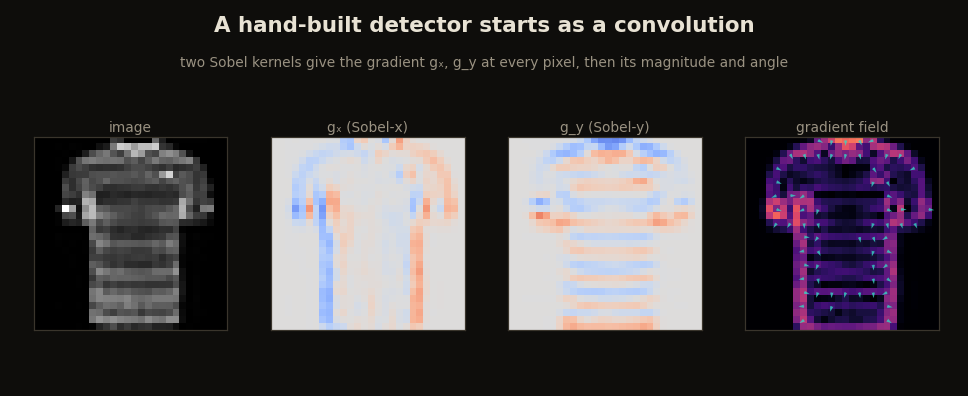
_conv call above, nothing more, a fixed convolution with no weights to learn. Rendered by scripts/render_handbuilt_gifs.py.The seven channels follow directly. Each oriented-edge channel is the gradient magnitude weighted by how close the edge angle sits to that channel’s orientation; the corner channel is the product of the two gradient directions, large only where both are strong. None of this has a parameter to fit.
@jax.jit
def features(imgs):                                     # [N,28,28] in [0,1] -> [N,343]
    gx, gy = _conv(imgs, SX), _conv(imgs, SY)
    mag = jnp.sqrt(gx ** 2 + gy ** 2) + 1e-6
    ang = jnp.mod(jnp.arctan2(gy, gx), jnp.pi)          # undirected edge angle
    d = jnp.abs(jnp.mod(ang[:, None] - CENTERS[None, :, None, None] + jnp.pi / 2, jnp.pi) - jnp.pi / 2)
    edges = jnp.clip(1 - d / (jnp.pi / NB), 0, 1) * mag[:, None]   # [N,NB,28,28]
    corner = (jnp.abs(gx) * jnp.abs(gy))[:, None]
    chans = jnp.concatenate([edges, corner], 1)         # [N,NCH,28,28]
    ...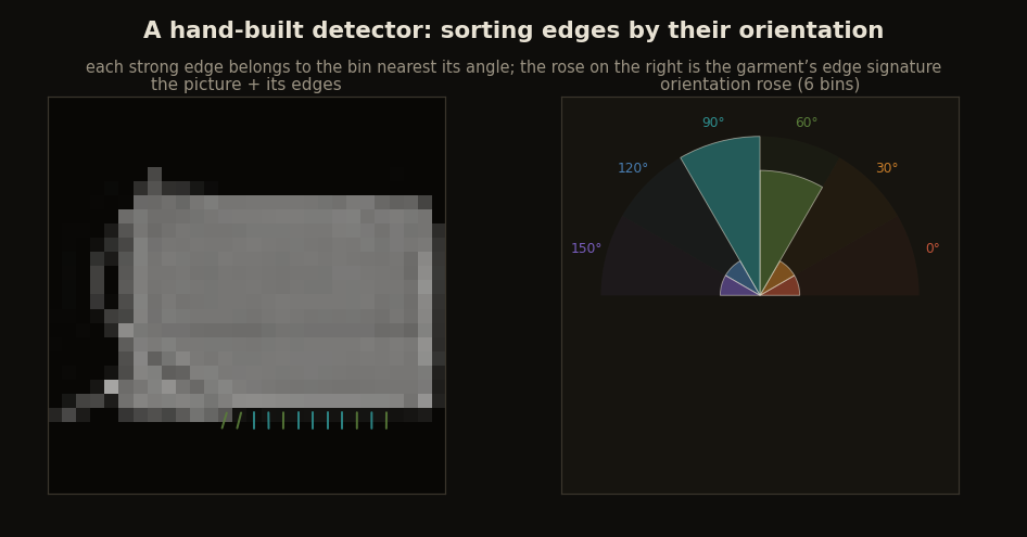
edges tensor above: gradient magnitude weighted by closeness to each of the six orientations, nothing fit. Rendered by scripts/render_handbuilt_gifs.py.The pooling, where the dimensions are named
The maps are full resolution, far more than a classifier wants, so each gets averaged over a 7-by-7 grid of patches. After that, the feature vector is one number for every (detector, patch) pair, 343 of them, and we L2-normalise each image so contrast does not matter.
    n = imgs.shape[0]; ps = 28 // GRID
    pooled = chans[:, :, :GRID * ps, :GRID * ps].reshape(n, NCH, GRID, ps, GRID, ps).mean((3, 5))
    V = pooled.reshape(n, -1)
    return V / (jnp.linalg.norm(V, axis=1, keepdims=True) + 1e-6)    # [N,343]
The whole extractor is @jax.jit and has no state. It is a function from an image to a fixed, named vector, which is exactly the thing the explainer means by “you built the representation.”
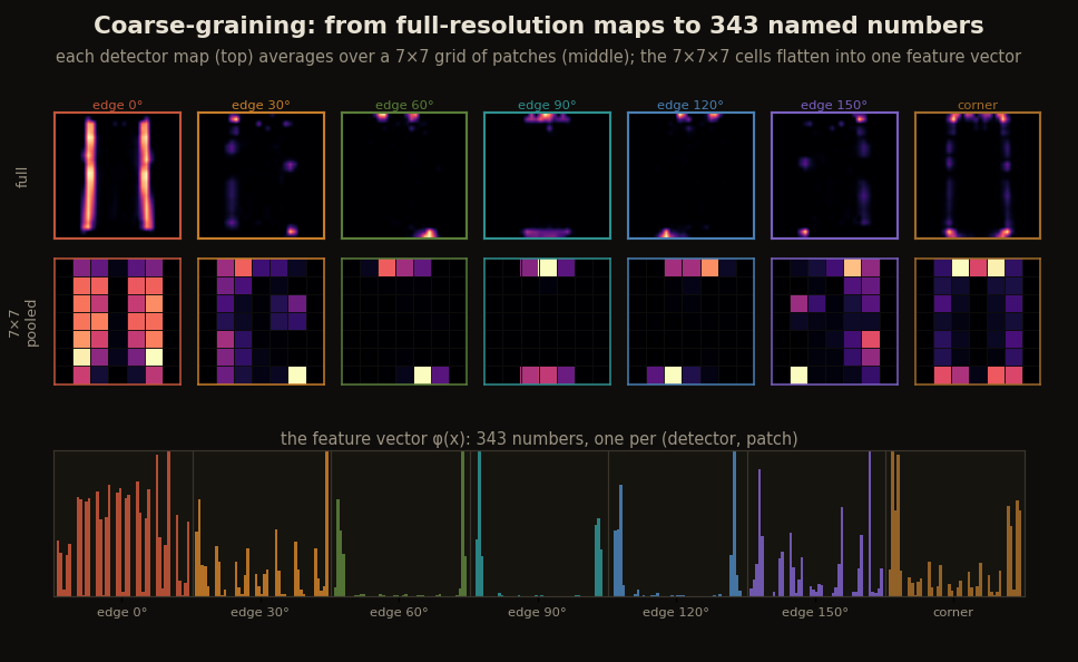
scripts/render_handbuilt_gifs.py.The head, as a parameter-free NNX module
What does a classifier nobody trains look like in a framework built for training? A perfectly ordinary module. The constructed Yat head from the earlier posts is written as Flax NNX so it slots into the same code as a trained network; the difference is that its variables are placed, not learned: the rows of W are k-means centroids of the training features, and A is a one-hot table sending each prototype’s vote to its class. The forward pass is the Yat kernel against every prototype, then the per-class maximum, then an argmax.
from flax import nnx

class YatHead(nnx.Module):
    """Prototypes W (k-means centroids), one-hot votes A, nearest-prototype vote."""
    def __init__(self, W, vote, b=0.5, eps=1.0):
        self.W = nnx.Variable(jnp.asarray(W))                       # [K, 343] prototypes
        self.A = nnx.Variable(jax.nn.one_hot(jnp.asarray(vote), 10))
        self.b, self.eps = b, eps

    def __call__(self, z):                                         # z: [N, 343] features
        dot = z @ self.W.value.T
        d2 = (z ** 2).sum(1, keepdims=True) + (self.W.value ** 2).sum(1) - 2 * dot
        ker = (dot + self.b) ** 2 / (d2 + self.eps)                # the Yat kernel
        scores = jnp.where(self.A.value.T[None].astype(bool), ker[:, None, :], -jnp.inf).max(-1)
        return scores.argmax(-1)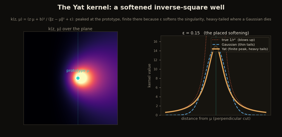
(dot + b)² / (d2 + eps), drawn out. Cut perpendicular to the prototype the kernel is a softened inverse-square well: a true 1/r² blows up at the prototype, a Gaussian dies too fast in the tails, and the Yat kernel sits between them, finite at the prototype because ε softens the singularity and heavy-tailed beyond it. The ε you place sets how sharp the well is. Rendered by scripts/render_handbuilt_gifs.py.There is no nnx.Param anywhere in it. nnx.Variable holds state that an optimizer would never touch, which is the right type for a thing you place by hand.
Building it and running it
The pieces assemble with no training step. Extract the features, z-score them, run k-means per class to get the prototypes, set the softening ε from the data’s own distance scale, and hand it all to the head. Even ε is placed, not learned: a tenth of the median squared feature-to-prototype distance, the knob the kernel-shape figure above turns.
Ftr, Fte = np.asarray(features(Xtr)), np.asarray(features(Xte))
mu, sd = Ftr.mean(0), Ftr.std(0) + 1e-6
Ftr, Fte = (Ftr - mu) / sd, (Fte - mu) / sd                        # z-score into the head's space

PER = 20; W, vote = [], []
for c in range(10):
    W += list(KMeans(PER, n_init=2, random_state=0).fit(Ftr[ytr == c][:2500]).cluster_centers_)
    vote += [c] * PER
W = np.array(W, 'float32'); vote = np.array(vote)

d2 = (Fte ** 2).sum(1, keepdims=True) + (W ** 2).sum(1) - 2 * Fte @ W.T
eps = float(np.median(d2) * 0.1)                                   # placed, like everything else

head = YatHead(W, vote, b=0.5, eps=eps)
pred = np.asarray(head(jnp.asarray(Fte)))
print(f"hand-built, no training anywhere: {100 * (pred == yte).mean():.1f}%")   # 83.3%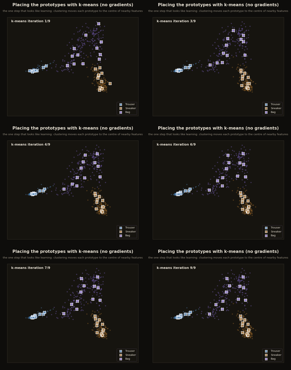
W: a few exemplars per class that the kernel votes against. Shown for three well-separated classes; the real head uses twenty per class. Rendered by scripts/render_handbuilt_gifs.py.It prints 83.3%, the same number the explainer’s interactive demo computes in the browser, because it is the same pipeline. The only place a fit happens at all is k-means, which is choosing where to place the prototypes, not learning a representation. Drop even that and the floor is still high: one plain mean per class, nearest mean wins, is two lines and reaches 75.6% (the check is in the explainer’s scripts/handbuilt_vision.py).
cen = np.stack([Ftr[ytr == c].mean(0) for c in range(10)])
print(100 * (((Fte[:, None] - cen[None]) ** 2).sum(2).argmin(1) == yte).mean())   # 75.6%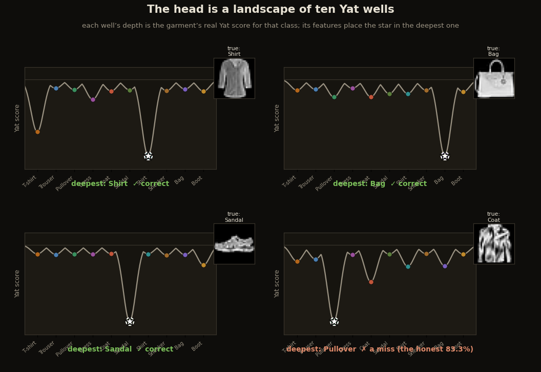
scores.argmax, nothing simulated. Three land in the right well; the fourth is a coat scoring highest for pullover, with coat the runner-up, which is exactly why the two confuse: the real 83.3%, not a perfect classifier. Rendered by scripts/render_handbuilt_gifs.py.What this leaves out
The k-means step is the one piece that looks like learning, and it is worth being precise: it is an unsupervised clustering of features the extractor already fixed, used only to pick prototype locations, with no gradient and no objective tied to accuracy. Everything upstream of it, the part that turns a picture into 343 numbers, is hand-written and frozen. That is the whole claim of the post made literal in code: a network whose every layer you can read, none of which was trained, that still classifies most of Fashion-MNIST correctly.
Hand-built oriented-gradient features are the HOG idea from Dalal and Triggs (2005); the prototype head from Chen et al. (2019); Fashion-MNIST from Xiao et al. (2017); the Yat kernel from Bouhsine (2026). The conceptual companion is You Don’t Even Have to Train the Features.
Cite as
Bouhsine, T. (). The Hand-Built Network, in JAX/Flax NNX. Records of the !mmortal Data Scientist. https://tahabouhsine.com/blog/handbuilt-features-jax-flax-nnx/
BibTeX
@misc{bouhsine2026handbuiltfeaturesjaxflaxnnx,
  author       = {Bouhsine, Taha},
  title        = {The Hand-Built Network, in JAX/Flax NNX},
  year         = {2026},
  month        = {jun},
  howpublished = {\url{https://tahabouhsine.com/blog/handbuilt-features-jax-flax-nnx/}},
  note         = {Blog post, Records of the !mmortal Data Scientist}
}References
- (2005). Histograms of Oriented Gradients for Human Detection. CVPR 2005.
- (2019). This Looks Like That: Deep Learning for Interpretable Image Recognition. NeurIPS 2019.arXiv:1806.10574
- (2017). Fashion-MNIST: a Novel Image Dataset for Benchmarking Machine Learning Algorithms. arXiv:1708.07747
- (2026). A Universal Reproducing Kernel Hilbert Space from Polynomial Alignment and IMQ Distance. arXiv:2605.03262