Editing a Network by Hand, in JAX/Flax NNX

The explainer argued that a Yat-kernel network is a list of prototype pictures, so you can teach it a class by adding pictures and make it forget one by deleting them, with no training. This is the implementation: build the network in Flax NNX, then watch teaching reduce to a jnp.concatenate and forgetting to a boolean mask. Every figure and number below is from a real run; the script is scripts/yat_editable_fmnist.py.

Prefer a notebook? Run the whole thing on Kaggle: the same code, block by block, with the math written out and every figure reproduced from a real run.

The layer, and what its rows are#

If teaching and forgetting are going to be array edits, the array has to be shaped for it: one prototype to a row, and nothing about a class smeared anywhere else. A Yat unit scores an input against a prototype $W_u$ with the kernel $(W_u^\top x + b)^2 / (\lVert x - W_u\rVert^2 + \varepsilon)$, a layer is a bank of them, and the readout rows record which class each prototype speaks for. The prototypes are the rows of W, each row’s class a row of A, and editing the network will turn out to be nothing more than editing those rows.

import jax, jax.numpy as jnp
from flax import nnx


class YatEdit(nnx.Module):
    """A bank of prototype rows W and their class assignments A. No activation function."""
    def __init__(self, W, A, *, b=0.5, eps=0.05):
        self.W = nnx.Param(jnp.asarray(W))            # [K, 784]  prototype pictures
        self.A = nnx.Param(jnp.asarray(A))            # [K, 10]   one-hot: row u's class
        self.b, self.eps = b, eps

    def kernel(self, x):                              # [n, K] resemblance of each input to each prototype
        dot = x @ self.W.value.T
        d2 = (x ** 2).sum(-1, keepdims=True) + (self.W.value ** 2).sum(-1) - 2 * dot
        return (dot + self.b) ** 2 / (d2 + self.eps)

    def __call__(self, x):                            # [n, 10] class scores
        k = self.kernel(x)                            # [n, K]
        per_class = jnp.where(self.A.value.T[None] > 0, k[:, None, :], -jnp.inf)
        return per_class.max(-1)                      # nearest prototype within each class

There is no nnx.Linear, no nonlinearity, and crucially no entanglement: prototype $u$ lives entirely in row $u$ of W and row $u$ of A. The decision rule is nearest-prototype within each class: class $c$ is scored by its best-matching row, $s_c(x) = \max_{u\,:\,\text{class}(u)=c} \phi_u(x)$, the mode='max' readout in scripts/yat_editable_fmnist.py and the rule behind every number in this post. The explainer writes the same structure as a pure linear readout, $s(x) = A^\top \phi(x)$, a sum over each class’s rows instead of a max; that view is worth keeping (it is what a linear layer can express, and it is where the field-superposition picture comes from), but it scores a few points lower, 68% against 79% at this scale. What every edit below actually rides on is shared by both readouts: class $c$‘s score is computed from class $c$‘s rows and no others, so appending rows extends one class and masking rows removes one, with zero cross-talk.

Build it by hand#

Before you can edit a network you need one to edit, and this one arrives without training. A few k-means centroids per class become the prototypes, each one’s readout row wired to one-hot, and no optimizer touches it.

import numpy as np, torchvision
from sklearn.cluster import KMeans

tr = torchvision.datasets.FashionMNIST("/tmp/fmnist", train=True, download=True)
te = torchvision.datasets.FashionMNIST("/tmp/fmnist", train=False, download=True)
X = tr.data.numpy().reshape(-1, 784).astype("float32") / 255.0; y = tr.targets.numpy()
Xte = te.data.numpy().reshape(-1, 784).astype("float32") / 255.0; yte = te.targets.numpy()

def prototypes(classes, per=20):
    W, lab = [], []
    for c in classes:
        W += list(KMeans(per, n_init=3, random_state=0).fit(X[y == c][:2500]).cluster_centers_)
        lab += [c] * per
    return np.array(W, "float32"), np.array(lab)

def build(classes, per=20):
    W, lab = prototypes(classes, per)
    A = np.eye(10)[lab].astype("float32")             # row u votes one-hot for class lab[u]
    return YatEdit(W, A)

model = build(range(10))
acc = float((jnp.argmax(model(jnp.asarray(Xte)), -1) == yte).mean())
print("zero-training accuracy:", round(acc * 100, 1))  # 79.4

The network classifies before any training, because it is a kernel machine from the first step. Geometrically, as the explainer frames it, the kernel’s $1/(\lVert x - W_u\rVert^2 + \varepsilon)$ is a softened inverse-square pull, so each prototype is a mass and classifying a point is letting it fall into the deepest basin it feels.

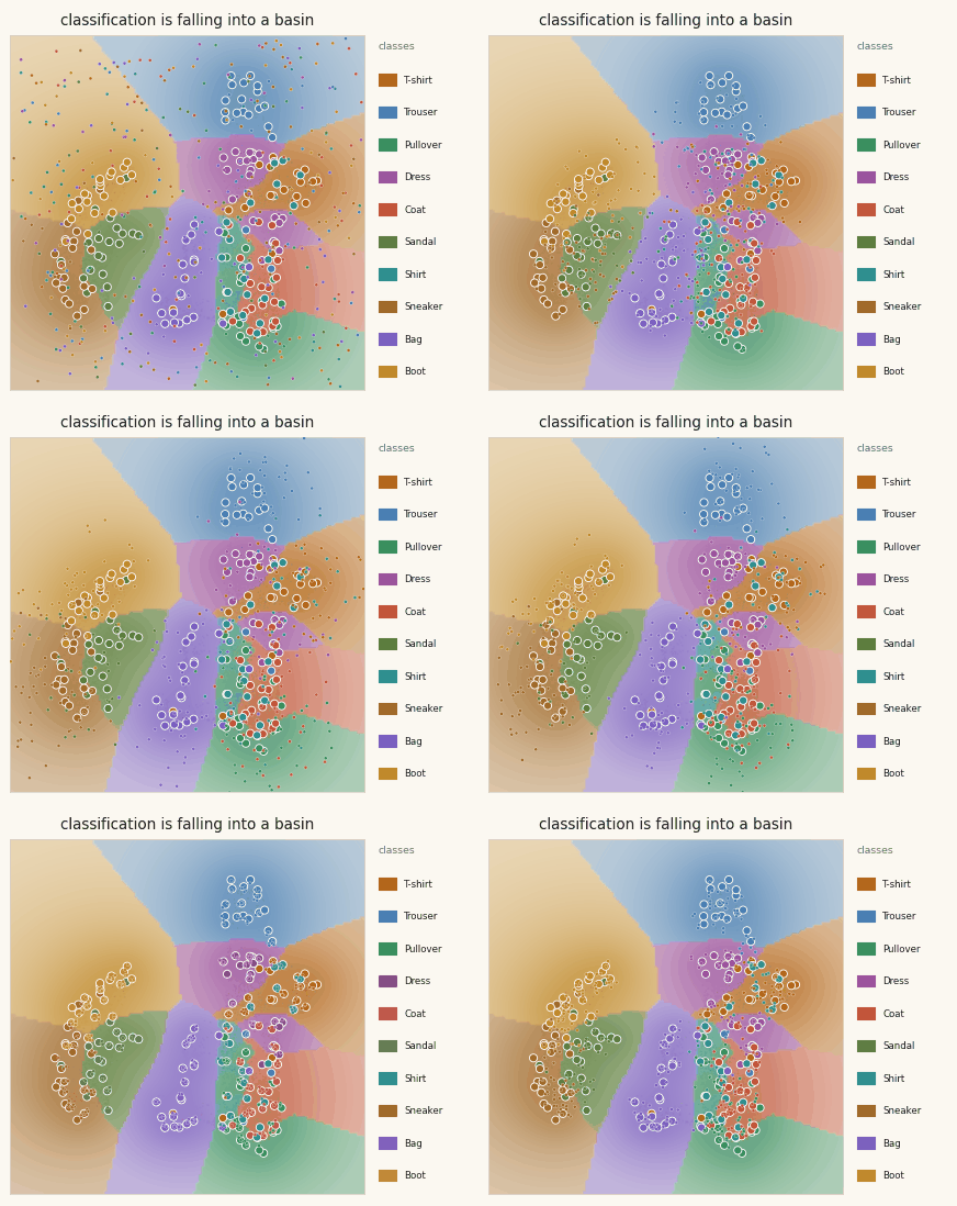
Everything from here is editing that field.

Teaching a class is a concatenate#

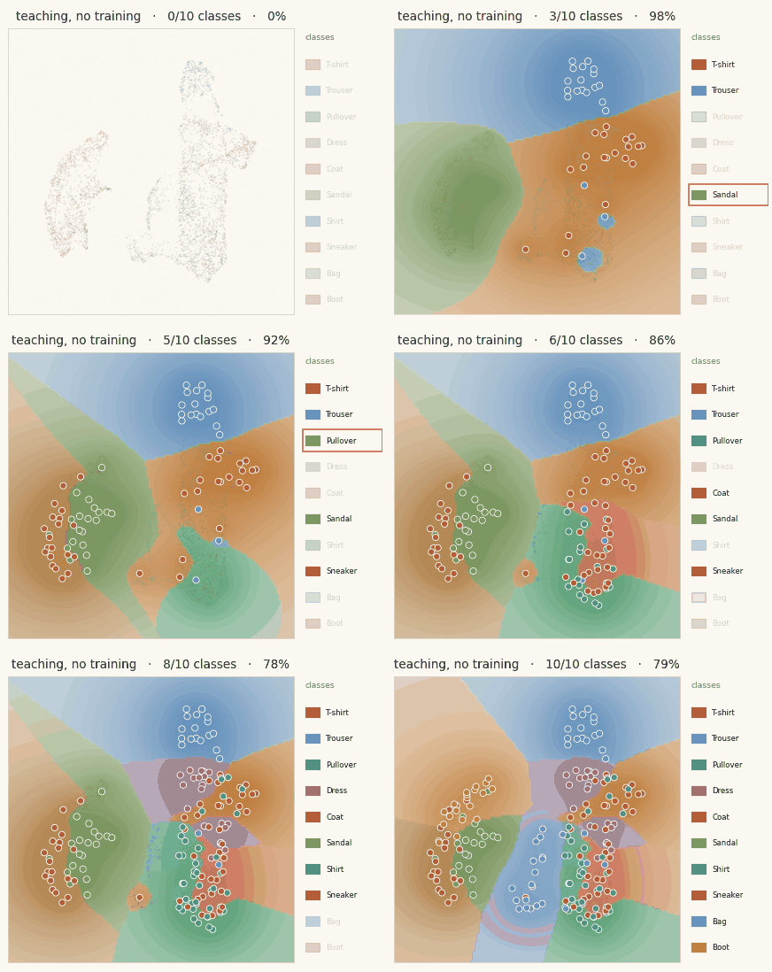
Teaching a deployed model a new class is supposed to be the dangerous direction, the one that quietly wrecks the classes it already knows. Here it is a stack of rows: build the new class’s prototypes and their one-hot readout rows, concatenate them on, and stop. That is the entire operation.

def add_class(model, c, per=20):
    Wc, _ = prototypes([c], per)
    Ac = np.eye(10)[[c] * per].astype("float32")
    model.W = nnx.Param(jnp.concatenate([model.W.value, jnp.asarray(Wc)], 0))
    model.A = nnx.Param(jnp.concatenate([model.A.value, jnp.asarray(Ac)], 0))
    return model

eight = build(range(8))                                # a network that has never seen Bag or Boot
mask8 = np.isin(yte, range(8))
print("8 classes:", round(float((jnp.argmax(eight(jnp.asarray(Xte[mask8])), -1) == yte[mask8]).mean()) * 100, 1))  # 77.8%

for c in (8, 9):                                       # teach Bag, then Boot, no gradient steps
    add_class(eight, c)

def recall(m, c):
    sel = yte == c
    return round(float((jnp.argmax(m(jnp.asarray(Xte[sel])), -1) == c).mean()) * 100)

print("Bag, Boot recall:", recall(eight, 8), recall(eight, 9))                                  # 95, 94
print("all 10:", round(float((jnp.argmax(eight(jnp.asarray(Xte)), -1) == yte).mean()) * 100, 1))  # 79.4
print("from scratch:", round(float((jnp.argmax(build(range(10))(jnp.asarray(Xte)), -1) == yte).mean()) * 100, 1))  # 79.4

The two classes it had never encountered are recognized at 95% and 94% the moment their rows are appended, and the classes it already knew barely move. The reason is one line of the algebra: the appended rows are one-hot at the new class $c$, so no other class’s score ever reads them. For every $c' \ne c$, $s_{c'}(x)$ is still the max (or the sum) over exactly the rows it had before, unchanged, while $s_c(x)$ alone gains the new candidates. Old-class scores are invariant under the concatenate. The headline is the last two lines: the network taught incrementally and the network built on all ten at once reach the same 79.4%, because a max, like a sum, does not remember the order its arguments arrived in. There is no penalty for incrementality, and no rehearsal buffer in sight.

Forgetting a class is a mask#

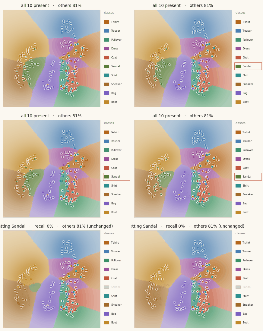
Unlearning is the same move in reverse. Find the rows assigned to the class, drop them. Because class $c$ lives only in the rows whose readout is one-hot at $c$, the deletion is exact, and this time we can hold the explainer to its promise: it said you could diff the weights afterward to prove nothing else moved, so snapshot them before the edit and check.

def forget_class(model, c):
    keep = np.asarray(model.A.value.argmax(-1)) != c   # rows NOT assigned to class c
    model.W = nnx.Param(model.W.value[keep])
    model.A = nnx.Param(model.A.value[keep])
    return model

m = build(range(10))
others = np.isin(yte, [c for c in range(10) if c != 5])
def acc_others(m):
    return round(float((jnp.argmax(m(jnp.asarray(Xte[others])), -1) == yte[others]).mean()) * 100, 1)

W0, A0 = np.asarray(m.W.value), np.asarray(m.A.value)  # snapshot before the edit
before = acc_others(m)
kept = A0.argmax(-1) != 5
forget_class(m, 5)                                     # forget Sandal

print("Sandal recall:", recall(m, 5))                  # 0
print("other 9 classes:", before, "->", acc_others(m)) # 81.1 -> 81.3
assert (np.asarray(m.W.value) == W0[kept]).all()       # surviving rows: bit-for-bit identical
assert (np.asarray(m.A.value) == A0[kept]).all()
print("weight diff over surviving rows:", float(np.abs(np.asarray(m.W.value) - W0[kept]).max()))  # 0.0

Sandal recall goes to 0: nothing in the network resembles a sandal anymore, so nothing can be labelled one. The other nine classes go from 81.1% to 81.3%, untouched, a hair better because the deleted rows are no longer around to occasionally steal a neighbour’s test image. And the two asserts are the unlearning proof, delivered: every surviving row of W and A is equal, bit for bit, to the row it was before the edit, a weight diff of exactly 0.0. The structural identity behind it: for $c' \ne 5$, $s_{c'}(x)$ is computed from class $c'$‘s rows alone, whether you take their max or their sum, and never indexed a Sandal row, so masking those rows out is a no-op on it. This is the line between exact unlearning and the approximate kind: not “we reduced its influence and hope,” but “the rows are not in the matrix, check.”

Why the edits are exact, in one sentence#

In an ordinary network the knowledge of a class is smeared across shared weights, so adding a class with gradient descent overwrites a little of every other class (catastrophic forgetting) and deleting one is a research problem (machine unlearning) whose exact baseline is to retrain from scratch. Here a class is a contiguous block of rows, so protecting it during an edit is do not index those rows and erasing it is index them out. jnp.concatenate and a boolean mask are the entire continual-learning and unlearning stack, because the architecture stores knowledge in a form you can address.

What this leaves out#

These rows are prototype pictures because the input space is pixel space; that is what makes the edits legible and is also the limit. Put the Yat kernel on top of learned features and a prototype becomes a feature-space exemplar, the ProtoPNet recipe (Chen et al., 2019), and those features still cost a training run, so the no-training claim narrows to no-training-of-the-head. That boundary, how much of a network you can construct rather than optimize, is the subject the explainer leaves open. What does not change is the object: a layer whose unit stores a row you can read, append, and delete, so that on images the row is a picture and editing the network is editing a list.

The prototype-network idea (“this looks like that”) is from Chen et al. (2019); machine unlearning from Bourtoule et al. (2021); Fashion-MNIST from Xiao et al. (2017); the Yat kernel from Bouhsine (2026). The conceptual companion is Your Network Is a List of Pictures. You Can Edit It..

@misc{bouhsine2026editanetworkjaxflaxnnx,
  author       = {Bouhsine, Taha},
  title        = {Editing a Network by Hand, in JAX/Flax NNX},
  year         = {2026},
  month        = {jun},
  howpublished = {\url{https://tahabouhsine.com/blog/edit-a-network-jax-flax-nnx/}},
  note         = {Blog post, Records of the !mmortal Data Scientist}
}