An Error Controller for a Trained Net, in JAX

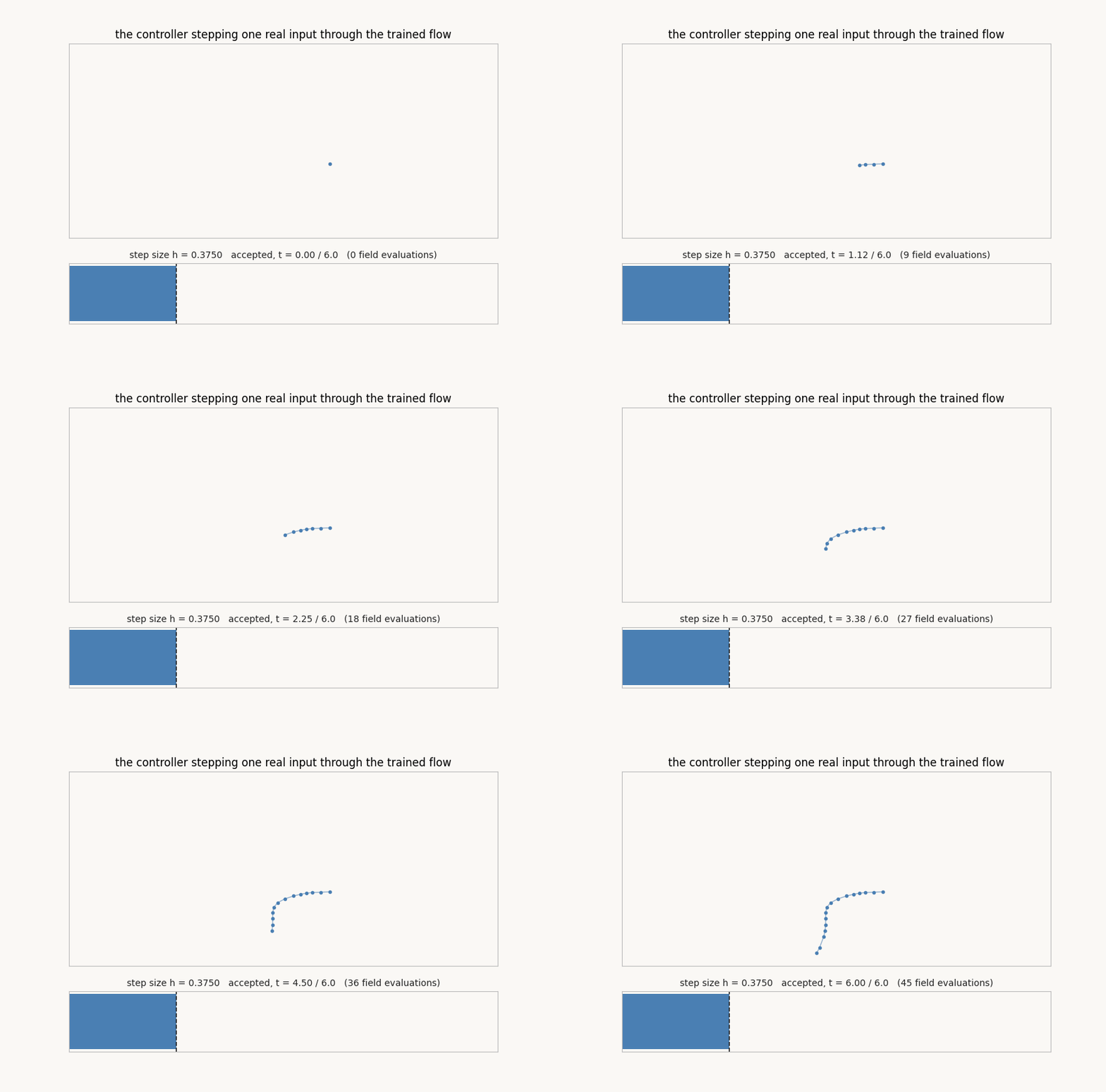
The controller here has no parameters and never sees a gradient. It takes one step, takes two half-steps, compares them, and either commits or halves and retries. Everything the explainer claims about depth becoming a dial after training follows from that comparison, run on a network trained once at fixed depth and never touched again. What is below is the renderer, the accounting that keeps rejected probes on the books, and the figures, all quoted from the Kaggle run (bundle kgl_blog-adaptive-v2).

Train fixed, render free#

Training is the previous post’s leapfrog net, sixteen kick-drift-kick steps of a learned potential as a lax.scan, trained end to end and never touched again. The controller is pure inference. Its unit of work is one leapfrog evaluation, and its whole intelligence is a comparison:

def render_adaptive(p, x, tol, h0=T_TOTAL / L_TRAIN, h_min=T_TOTAL / 4096):
    z = np_affine(x[None], p["enc"])
    q, pm = z[:, :DIM], z[:, DIM:]
    t, h, work, accepted = 0.0, h0, 0, 0
    while t < T_TOTAL - 1e-9:
        h = min(h, T_TOTAL - t)
        q1, p1 = np_leap(p, h, q, pm)                    # one h step
        qh, ph = np_leap(p, h / 2, q, pm)                # two h/2 steps
        q2, p2 = np_leap(p, h / 2, qh, ph)
        work += 3
        err = float(np.max(np.abs(np.concatenate([q1 - q2, p1 - p2], 1))))
        if err > tol and h > h_min:
            h = h / 2                                     # too sharp: refine, retry
            continue
        q, pm = q2, p2                                    # accept the finer render
        accepted += 2                                     # two committed h/2 steps
        t += h
        if err < tol / 4:
            h = min(h * 2, T_TOTAL / 4)                   # gentle: stride out
    lg = np_affine(np.concatenate([q, pm], 1), p["dec"])[0]
    return lg, work, accepted

Two counters, deliberately kept apart. work counts every leapfrog evaluation, including the probes of steps that were rejected, because that is what the controller actually costs; accepted counts only committed steps, the rendered resolution. The explainer’s efficiency claims use work; the power law lives in accepted. Conflating them flatters the method by a factor of about two, so the run keeps both.

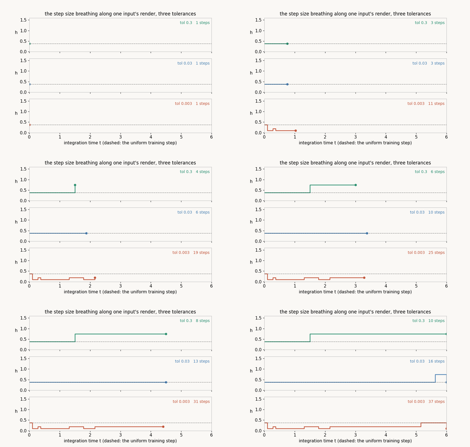
The same decisions, seen as the step size breathing in time, once per tolerance:

The dial in numbers#

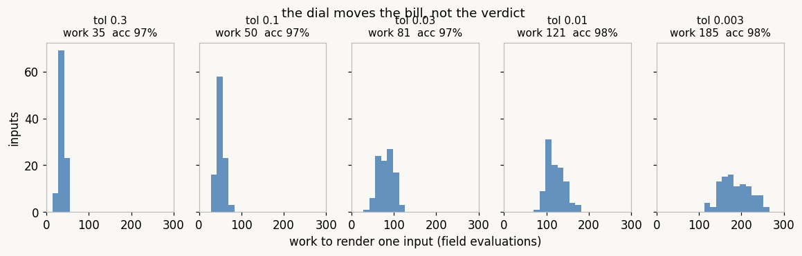
Sweeping the tolerance re-renders the same inputs at five precisions. The work histogram moves; the verdicts do not:

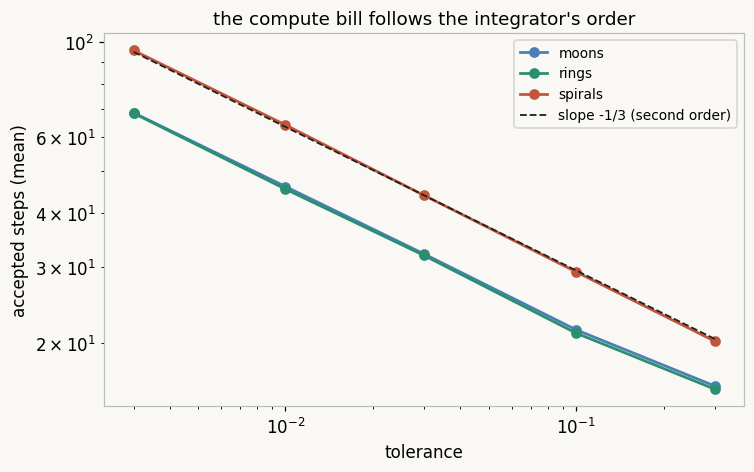
The mean of that moving histogram is lawful. Accepted steps against tolerance on log-log axes, all three datasets, with the second-order method’s slope drawn once:

Where the money goes#

The run’s most useful negative result is the geography of effort. Rendering every point of the input plane at one tolerance and coloring by work:

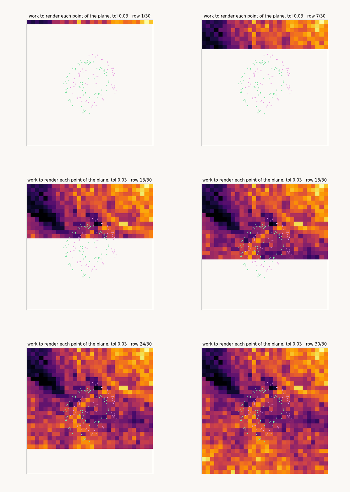
The explainer draws the moral; the implementation note is just that this field costs nothing to explore, because the controller is inference-only: no gradient, no retraining, one while-loop per pixel.

Every number above is from one run on Kaggle (bundle kgl_blog-adaptive-v2); the figures are rendered from the bundle’s exported seed-0 weights, replaying the identical controller arithmetic.

@misc{bouhsine2026depthondemandjaxflaxnnx,
  author       = {Bouhsine, Taha},
  title        = {An Error Controller for a Trained Net, in JAX},
  year         = {2026},
  month        = {jul},
  howpublished = {\url{https://tahabouhsine.com/blog/depth-on-demand-jax-flax-nnx/}},
  note         = {Blog post, Records of the !mmortal Data Scientist}
}