Building the Energy-Conserving Net in JAX/Flax NNX

The explainer trains a network whose motion is derived from a learned scalar, so the scalar is conserved by construction, then turns the same idea into a residual block. This is the implementation: both field models and the leapfrog classifier as Flax NNX modules, depth as a lax.scan, and the structural claims re-checked from scratch. The published numbers are from scripts/hamiltonian_net.py on Kaggle; every code block below runs as written in scripts/hamiltonian_nnx_check.py, and every figure is rendered from the real run by scripts/render_hamiltonian_gifs.py.

One scalar, two outputs for free#

The whole trick fits in a class definition. A plain field model maps a state to two numbers and both are free. The HNN maps a state to one number and manufactures the two outputs from its gradient, rotated a quarter turn:

class HNNField(nnx.Module):
    """One scalar H(q, p); the field is (dH/dp, -dH/dq)."""

    def __init__(self, hidden=64, *, rngs):
        self.l1 = nnx.Linear(2, hidden, rngs=rngs)
        self.l2 = nnx.Linear(hidden, hidden, rngs=rngs)
        self.l3 = nnx.Linear(hidden, 1, rngs=rngs)

    def energy(self, qp):                      # (..., 2) -> (...,)
        h = jnp.tanh(self.l1(qp))
        h = jnp.tanh(self.l2(h))
        return self.l3(h)[..., 0]

    def __call__(self, qp):                    # the symplectic gradient
        g = jax.vmap(jax.grad(lambda s: self.energy(s)))(qp)
        return jnp.stack([g[:, 1], -g[:, 0]], axis=1)

jax.grad through the module is the entire implementation of “derive the motion from the energy”. The control is the same MLP with two output units and no scalar anywhere:

class PlainField(nnx.Module):
    def __init__(self, hidden=64, *, rngs):
        self.l1 = nnx.Linear(2, hidden, rngs=rngs)
        self.l2 = nnx.Linear(hidden, hidden, rngs=rngs)
        self.l3 = nnx.Linear(hidden, 2, rngs=rngs)

    def __call__(self, qp):
        h = jnp.tanh(self.l1(qp))
        h = jnp.tanh(self.l2(h))
        return self.l3(h)

Both fit the same pendulum arrows, $(\dot q, \dot p) = (p, -\sin q)$ sampled on a band of states, with the same loop:

def fit(model, S, T, steps=1500, lr=1e-3):
    opt = nnx.Optimizer(model, optax.adam(lr), wrt=nnx.Param)

    @nnx.jit
    def step(model, opt):
        loss, grads = nnx.value_and_grad(lambda m: jnp.mean((m(S) - T) ** 2))(model)
        opt.update(model, grads)
        return loss

    for _ in range(steps):
        loss = step(model, opt)
    return float(loss)

In the check run both models fit the arrows well (plain 3.4e-04, HNN 1.1e-04). On the fit, nothing distinguishes them. The distinction is dynamical, so integrate.

Roll both out and watch the invariant#

RK4 as a lax.scan, recording the state so we can price each model’s energy behavior:

def rollout_energy(model, q0=1.6, p0=0.0, dt=0.05, n=600):
    def rk4(s, _):
        k1 = model(s); k2 = model(s + 0.5 * dt * k1)
        k3 = model(s + 0.5 * dt * k2); k4 = model(s + dt * k3)
        s2 = s + (dt / 6) * (k1 + 2 * k2 + 2 * k3 + k4)
        return s2, s2[0]

    s0 = jnp.array([[q0, p0]], dtype=jnp.float32)
    _, traj = jax.lax.scan(rk4, s0, None, length=n)
    E = 0.5 * traj[:, 1] ** 2 + (1 - jnp.cos(traj[:, 0]))
    E0 = 0.5 * p0 ** 2 + (1 - np.cos(q0))
    return float(jnp.max(jnp.abs(E - E0)) / E0)

In the check run the plain field drifts 6.4% of the starting energy over the rollout; the HNN holds within 0.4%. The published run’s longer rollout is the figure below, drawn from the exported trajectories.

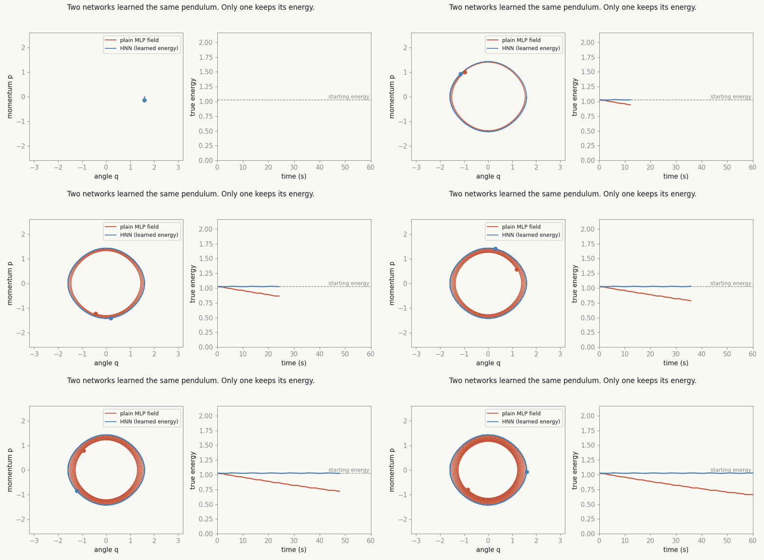
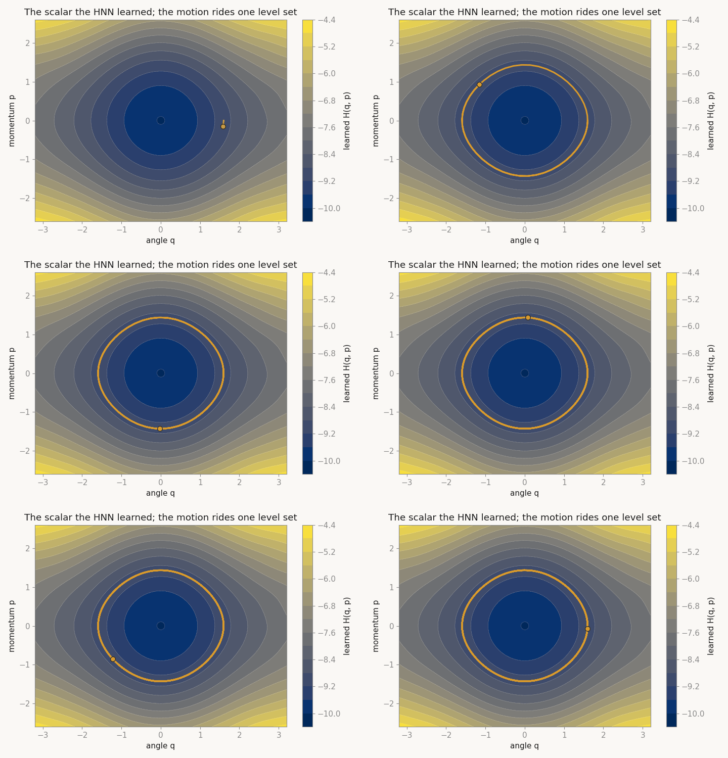
What the HNN learned is worth looking at directly: one scalar over phase space whose level sets are the orbits.

The leapfrog classifier#

The explainer’s second move turns the integrator into an architecture. Hidden state $(q, p)$, and the only learned thing in the block is a scalar potential $V_\theta(q)$; one layer is one kick-drift-kick step. In NNX, with depth as a lax.scan over the shared block:

class LeapfrogNet(nnx.Module):
    """Hidden state (q, p); one shared block = one leapfrog step of V(q)."""

    def __init__(self, hidden=32, *, rngs):
        self.enc = nnx.Linear(2, 2 * DIM, rngs=rngs)
        self.v1 = nnx.Linear(DIM, hidden, rngs=rngs)
        self.v2 = nnx.Linear(hidden, DIM, rngs=rngs)
        self.dec = nnx.Linear(2 * DIM, 2, rngs=rngs)

    def potential(self, q):                    # scalar V per row
        return (self.v2(jnp.tanh(self.v1(q)))).sum(axis=-1)

    def grad_v(self, q):
        return jax.vmap(jax.grad(lambda qi: self.potential(qi[None])[0]))(q)

    def __call__(self, x, L=16):
        h = T_TOTAL / L
        z = self.enc(x)
        q, p = z[:, :DIM], z[:, DIM:]

        def step(carry, _):
            q, p = carry
            p = p - 0.5 * h * self.grad_v(q)   # kick
            q = q + h * p                      # drift
            p = p - 0.5 * h * self.grad_v(q)   # kick
            return (q, p), None

        (q, p), _ = jax.lax.scan(step, (q, p), None, length=L)
        return self.dec(jnp.concatenate([q, p], axis=1))

Three things to notice. The step size is $h = T/L$ with $T$ fixed, so depth is a resolution, not a budget: net(x, L=64) runs the same trained weights at four times finer steps. The block is shared across depth, so a deeper call invents no new parameters. And the training loop is completely ordinary:

net = LeapfrogNet(rngs=nnx.Rngs(0))
opt = nnx.Optimizer(net, optax.adam(3e-3), wrt=nnx.Param)

@nnx.jit
def step(net, opt):
    def loss_fn(m):
        return optax.softmax_cross_entropy_with_integer_labels(m(X), y).mean()
    loss, grads = nnx.value_and_grad(loss_fn)(net)
    opt.update(net, grads)
    return loss

In the check run this reaches 100% on held-out moons at its training depth and 100% again at four times that depth, with the learned energy $E_\theta = \tfrac12\|p\|^2 + V_\theta(q)$ oscillating in a bounded band through the layers rather than trending anywhere. The published three-seed comparison against the parameter-matched plain net is in the explainer’s table, along with the run’s cleanest structural result: the energy band shrinks sixteen-fold when the step halves twice, the $h^2$ signature of a second-order symplectic integrator measured inside a trained classifier. Here is the hidden state itself, from the exported seed-0 weights.

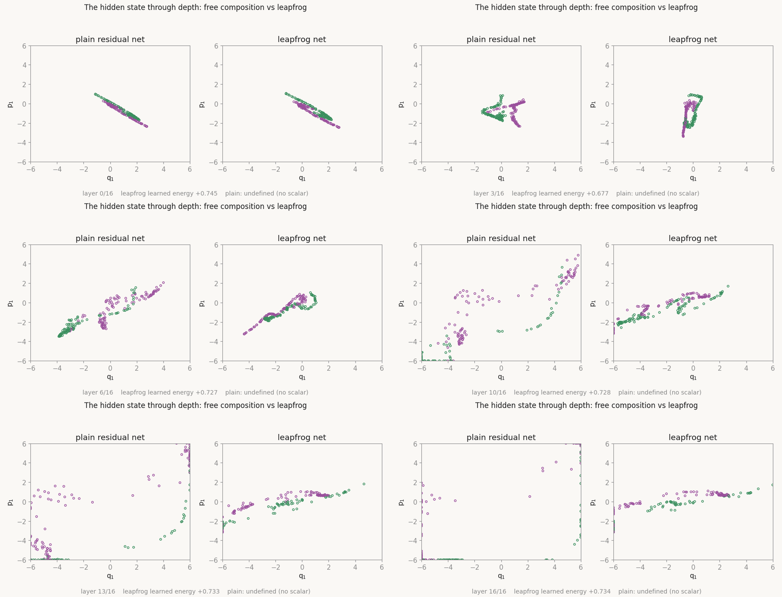
Depth as a dial you can turn after training#

The payoff figure re-runs both trained networks at depths they never trained at, from 4 to 128 layers, and draws each decision boundary as the sweep passes through.

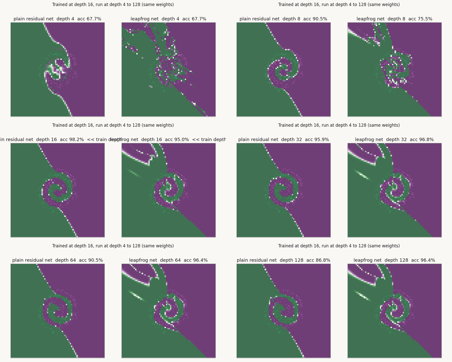
The one-line summary of the whole build: put the learnable thing one derivative inside the dynamics, and the dynamics inherit a law no loss term has to police.

Published numbers: scripts/hamiltonian_net.py (Kaggle, three seeds; bundle scripts/results/kgl_blog-hamiltonian-v1/). The code blocks in this post run as written in scripts/hamiltonian_nnx_check.py (Kaggle, bundle scripts/results/kgl_blog-hamiltonian-nnx-check/). Figures: scripts/render_hamiltonian_gifs.py from the run bundle.

@misc{bouhsine2026anetworkthatconservesenergyjaxflaxnnx,
  author       = {Bouhsine, Taha},
  title        = {Building the Energy-Conserving Net in JAX/Flax NNX},
  year         = {2026},
  month        = {jul},
  howpublished = {\url{https://tahabouhsine.com/blog/a-network-that-conserves-energy-jax-flax-nnx/}},
  note         = {Blog post, Records of the !mmortal Data Scientist}
}