Lazy Training a Yat Network in JAX/Flax NNX

July 26, 2026 · 7 min read

#kernels #random-features #lazy-training #yat #jax #flax #nnx #implementation

Part 13 of 13The Prototype Network

Explainer companionHow Many Random Neurons Buy a Trained One?Want the full intuition first? This is the runnable companion to the explainer.Read the explainer

The explainer freezes a bank of random Yat units and asks how many frozen neurons buy a trained one. This is the implementation side: the layer, the freeze, the fairness protocol, and the telemetry, all from scripts/yat_lazy.py, the script the Kaggle bundles ran (kgl_blog-yatlazy-v1 and its audits); figures are rendered from the bundles by scripts/render_lazy_gifs.py.

The layer, and how to freeze only part of a model

The hidden layer is the series’ standard Yat bank: prototypes as parameters, the kernel as the nonlinearity, both scalars stored raw behind a softplus so admissibility is structural:

class YatLayer(nnx.Module):
    def __init__(s, d_in, m, *, rngs, init="lecun"):
        if init == "lecun":
            W0 = nnx.initializers.lecun_normal()(rngs.params(), (m, d_in))
        else:  # data-seeded: m random training images as prototypes
            idx = jax.random.choice(rngs.params(), len(Xtr), (m,), replace=False)
            W0 = jnp.asarray(Xtr)[idx]
        s.W = nnx.Param(W0)
        s.log_b = nnx.Param(jnp.full((), jnp.log(jnp.expm1(0.5))))
        s.log_eps = nnx.Param(jnp.full((), jnp.log(jnp.expm1(0.5))))

    def __call__(s, x):
        b = jax.nn.softplus(s.log_b.value)
        eps = jax.nn.softplus(s.log_eps.value)
        dot = x @ s.W.value.T
        d2 = (jnp.sum(x * x, -1, keepdims=True)
              + jnp.sum(s.W.value ** 2, -1) - 2 * dot)
        return (dot + b) ** 2 / (jnp.maximum(d2, 0.0) + eps)

Freezing is not a stop_gradient scattered through the forward pass; in NNX it is a filter. The frozen arms declare that only the head’s parameters are trainable, hand that filter to the optimizer and to value_and_grad, and the bank never sees an update:

trainable = (nnx.All(nnx.Param, nnx.PathContains("head"))
             if frozen else nnx.Param)
opt = nnx.Optimizer(model, optax.adamw(lr, weight_decay=1e-4), wrt=trainable)

loss, grads = nnx.value_and_grad(
    loss_fn, argnums=nnx.DiffState(0, trainable))(model)
opt.update(model, grads)

Everything else, data order, batches, epochs, evaluation, is shared across all seven arms; the only differences are the init (lecun or data-seeded), the nonlinearity (Yat, Gaussian, or ReLU), and that one filter.

One neuron, one sample, watched

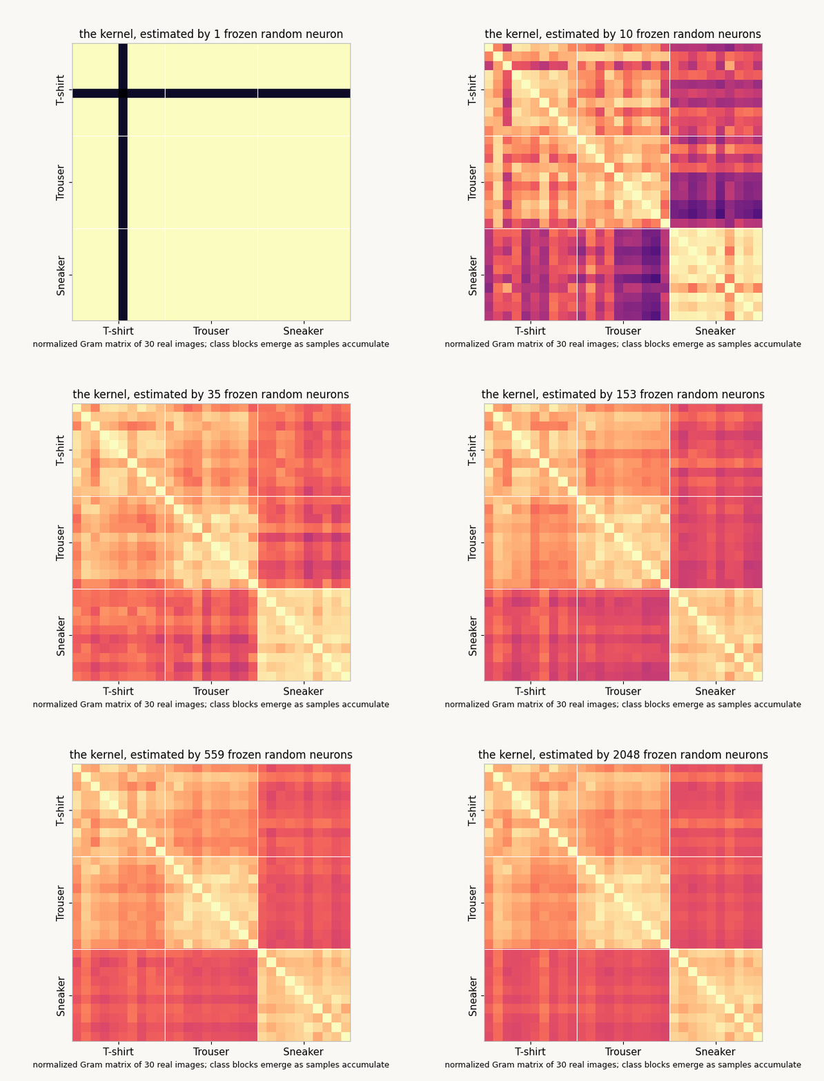
The explainer’s central reading is that a frozen random bank is a Monte Carlo estimate of a kernel, one neuron per sample. Here is the estimate concentrating, on thirty real images from three classes: at one neuron the Gram matrix is noise, and the class blocks condense out of it as neurons accumulate:

A thirty-by-thirty Gram matrix heatmap crystallizing from noise into a clear three-block class structure as the counter of random neurons climbs from one to two thousand — The normalized Gram matrix of 30 Fashion-MNIST images (ten T-shirts, ten trousers, ten sneakers) under a growing bank of frozen random Yat units, recomputed at every frame from the real features. One neuron gives a random similarity; two thousand give the random-feature kernel’s verdict, same-class blocks bright, cross-class blocks dark. Nothing trains anywhere in this figure; the structure is entirely the initializer’s kernel, emerging at the Monte Carlo rate.

The readout does the work

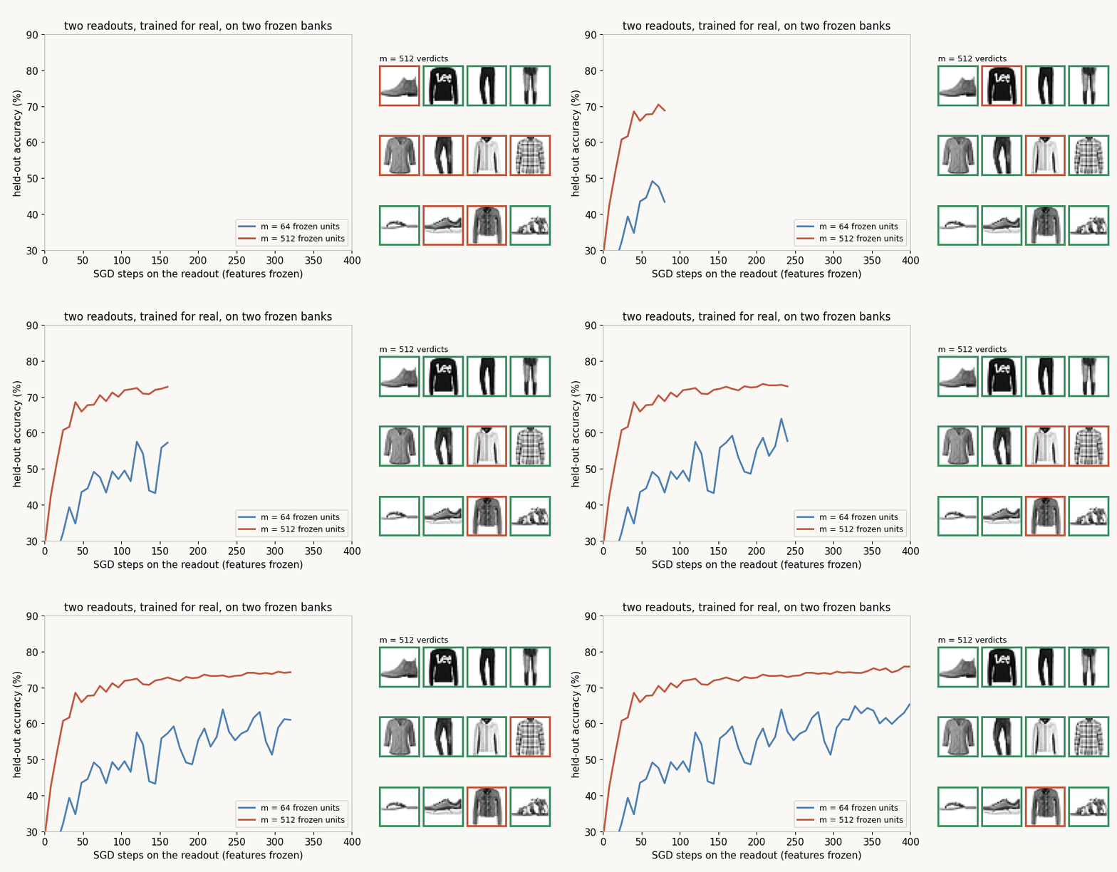
With features frozen, training is a convex fit, and it looks like one. Two banks, 64 and 512 units, each with a linear readout trained by Adam inside the render script on 10,000 real images:

Two accuracy curves rising through SGD steps, the 512-unit bank clearly above the 64-unit bank, while a grid of twelve test garments flips from orange to green borders as the larger readout learns — Two readouts training for real on frozen banks, accuracy through SGD steps; the thumbnails show the 512-unit readout’s live verdicts on twelve test garments. Both climb fast (the problem is convex), both plateau (the wall is the bank, not the optimizer), and the bigger bank’s wall is higher. This is the companion’s small-scale rendition of the explainer’s in-page panel; the full-scale numbers come from the Kaggle grid below.

The ladder, the law, and the rates that found them

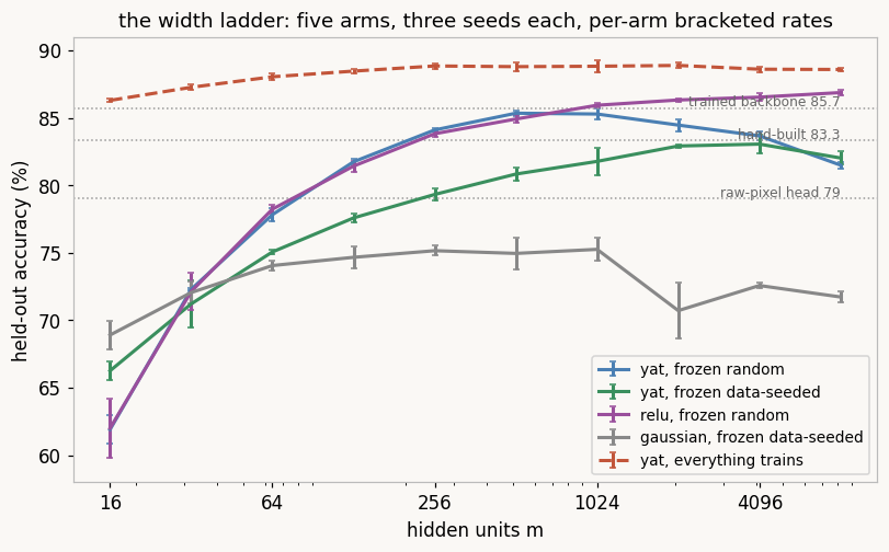
The full grid is ten widths by seven arms by three seeds, and its fairness protocol is worth quoting because the arms wanted wildly different learning rates. Each arm brackets its own rate at m = 256 before running its width grid:

GRIDS = {True: [3e-3, 1e-2, 3e-2], False: [3e-2, 1e-1, 3e-1, 1.0]}
for lr in GRIDS[arm in TRAINED_ARMS]:
    cells.append(run(arm, 256, 0, lr=lr))
chosen[arm] = max(cells, key=lambda r: r["best_acc"])["lr"]

arm	bracketed rate	best of the sweep
yat, frozen random	1.0	85.3 at m = 512
yat, frozen data-seeded	0.3	83.0 at m = 4096
relu, frozen random	0.03	86.9 at m = 8192
gaussian, frozen data-seeded	0.03	75.2 at m = 1024
yat, trained	0.01	88.9 at m = 2048

The convex readouts tolerate rates ten to a hundred times hotter than the full network, and the frozen Yat bank’s tiny feature scale demands the hottest of all. The scoreboard and the post’s headline law, as static figures:

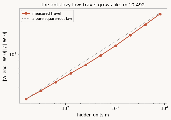
Accuracy against width for five arms with seed error bars, three dotted reference rungs, and the trained arm's dashed curve above all frozen curves at every width — The width ladder: ten widths are ten facts, so this is a chart, not an animation. The trained arm’s dashed curve enters at 86.3 with sixteen units, above every frozen point in the sweep.

A log-log plot of relative prototype movement against width, a straight line following a square-root law next to a dotted reference — The anti-lazy law on log axes: relative prototype travel against width, next to a pure square-root reference. The measured slope is 0.49 with R-squared 0.998.

The movement statistic itself is three lines of telemetry, kept per unit so the median and the maximum can disagree (they barely do):

Wf = np.asarray(model.feat.W.value)
out["w_move_rel"] = float(np.linalg.norm(Wf - W0) / np.linalg.norm(W0))
mv = np.linalg.norm(Wf - W0, axis=1) / np.linalg.norm(W0, axis=1)
out["w_move_median"], out["w_move_max"] = float(np.median(mv)), float(mv.max())

Watch the prototypes travel

The trajectory bundle (kgl_blog-yatlazy-traj) retrains three arms at m = 64 with a snapshot of the first sixteen prototypes at every epoch, so the anti-lazy law can be watched instead of summarized:

Two rows of eight prototype images evolving across training epochs: the random-init row drifts from static toward ghostly garment textures while the data-init row's garments roughen but survive — The run’s actual prototype snapshots, epoch by epoch, same training, two initializations. The random-init row travels almost five times its initialization norm and drifts toward ghostly, garment-textured objects without ever becoming the readable pictures data-seeding gives for free; the data-init row roughens and keeps its garments. Movement and legibility are different quantities, which is the gallery form of the explainer’s point that legibility is decided at initialization.

Two panels drawing through training epochs: median prototype travel climbing steeply for the random-init yat arm while the two data-seeded arms stay near one, and the corresponding accuracy curves with the random-init arm on top — Median prototype travel and held-out accuracy through the trajectory run’s 24 epochs, drawn in training time. The random-init Yat arm keeps traveling all run and finishes on top (88.7); the data-seeded Yat and Gaussian arms barely move (about 1x and 0.8x) and finish below it (87.1, 84.5). The arm that travels furthest wins, and the Gaussian, which the classical literature expects to be the stiffest, moves least and gains least.

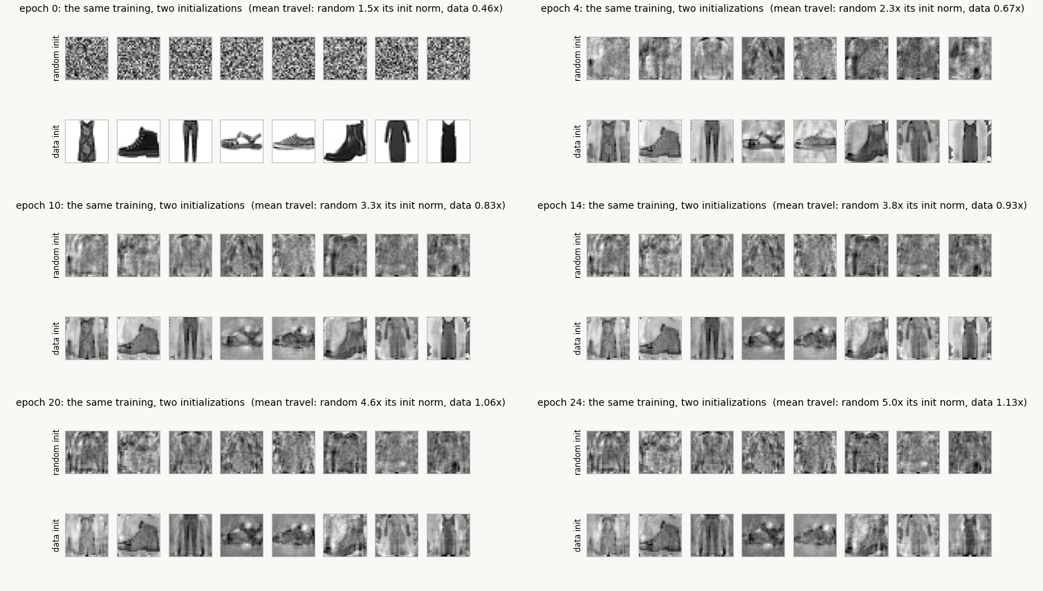
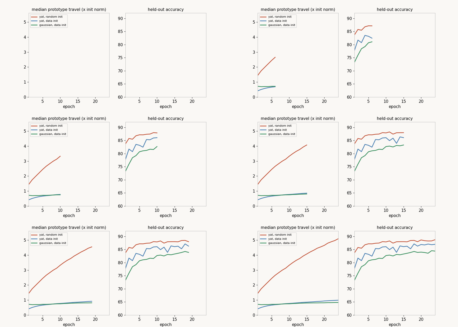
Every number is from scripts/yat_lazy.py on Kaggle: the main grid kgl_blog-yatlazy-v1 (seven arms, widths 16 to 8,192, three seeds, per-arm bracketed rates), the budget audits kgl_blog-yatlazy-bigm and -bigm2, the rate audits -lrsweep and -lrsweep2, and the trajectory bundle -traj (m = 64, 24 epochs, per-epoch snapshots). The Gram and readout-race figures are computed by scripts/render_lazy_gifs.py from raw Fashion-MNIST with the run’s exact layer math; the analysis and the redundancy measurement live in scripts/export_yat_lazy_viz.py.

Cite as

Bouhsine, T. (2026, July 26). Lazy Training a Yat Network in JAX/Flax NNX. Records of the !mmortal Data Scientist. https://tahabouhsine.com/blog/lazy-training-jax-flax-nnx/

BibTeX

@misc{bouhsine2026lazytrainingjaxflaxnnx,
  author       = {Bouhsine, Taha},
  title        = {Lazy Training a Yat Network in JAX/Flax NNX},
  year         = {2026},
  month        = {jul},
  howpublished = {\url{https://tahabouhsine.com/blog/lazy-training-jax-flax-nnx/}},
  note         = {Blog post, Records of the !mmortal Data Scientist}
}

References

Rahimi, A., Recht, B. (2007). Random Features for Large-Scale Kernel Machines. NeurIPS 2007.
Chizat, L., Oyallon, E., Bach, F. (2019). On Lazy Training in Differentiable Programming. NeurIPS 2019.arXiv:1812.07956

The layer, and how to freeze only part of a model#

One neuron, one sample, watched#

The readout does the work#

The ladder, the law, and the rates that found them#

Watch the prototypes travel#