Solving It and Descending It, in JAX/Flax NNX

The explainer took one Mercer kernel and fitted it twice, once by the classical exact solve and once by plain gradient descent, and found the two machines agree at r = 0.95 before the descended one walks through the walls the solved one dies at. This is the machinery underneath that claim: the kernel and its Gram matrix, the Cholesky solve, the same kernel as a Flax NNX module under Optax AdamW, the timing loop that measured the wall, the minibatch run through 511,012 rows, and the conv trunk the solve can never train. Every number is from the Kaggle runs of scripts/kernel_solve_wall.py.

One kernel, four lines#

Everything in the battery, both fitting procedures included, reduces to evaluating one function between pairs of points. The Yat kernel (Bouhsine, 2026) is squared alignment over softened squared distance, so its Gram matrix is a dot-product table and a distance table combined elementwise:

def yat_gram(A, B, eps=EPS):
    """k(a,b) = (a.b)^2 / (||a-b||^2 + eps), float64 on CPU by default."""
    dot = A @ B.T
    sq = (A * A).sum(1)[:, None] + (B * B).sum(1)[None, :] - 2.0 * dot
    return (dot * dot) / (np.maximum(sq, 0.0) + eps)

The np.maximum(sq, 0.0) guards the one numerical trap: expanding $\lVert a-b\rVert^2$ as $\lVert a\rVert^2 + \lVert b\rVert^2 - 2\,a^\top b$ can go microscopically negative in floating point, and a negative distance under the softening would poison the Cholesky factorization downstream. Both machines in this post call this same function, or compute exactly this expression inside their forward pass, which is what “the same kernel, fitted twice” means at the code level.

The exact machine is a factorization#

The classical fit is kernel ridge regression: build the full Gram over the training set, add the ridge to the diagonal, factorize, back-substitute. Prediction is another Gram, this time between queries and every training point, times the solved coefficients.

def solve_krr(Xtr, ytr, lam, eps=EPS, dtype=np.float64):
    """Exact Yat-kernel ridge: alpha = (K + lam I)^-1 y. Returns predict fn."""
    from scipy.linalg import cho_factor, cho_solve

    K = yat_gram(Xtr.astype(dtype), Xtr.astype(dtype), eps).astype(dtype)
    K[np.diag_indices_from(K)] += lam
    cf = cho_factor(K, lower=True)
    alpha = cho_solve(cf, ytr.astype(dtype))

    def predict(X, chunk=4096):
        outs = []
        for i in range(0, len(X), chunk):
            outs.append(yat_gram(X[i:i + chunk].astype(dtype), Xtr.astype(dtype), eps) @ alpha)
        return np.concatenate(outs)

    return predict, alpha

Cholesky rather than a generic solve because the kernel is positive definite and the ridge makes the system strictly so; the factorization is the $O(n^3)$ step the whole post is about. Notice what the machine keeps: Xtr itself, forever, because prediction needs a kernel evaluation against every training point.

The solve has two hyperparameters, and one of them is the kernel. eps sits in the denominator the way a Gaussian bandwidth sits in an exponent, so it is selected the same way, jointly with the ridge on a validation set, with candidates seeded by the median squared distance of the data:

def pick_lam_eps(Xtr, ytr, Xva, yva, lams=(1e-3, 1e-2, 1e-1, 1.0), epss=None):
    """eps is the kernel's bandwidth; select it on val jointly with the ridge,
    exactly as one would a Gaussian bandwidth. The descended net then uses the
    SAME eps, so both fits carry the same kernel."""
    if epss is None:
        med = median_sq_dist(Xtr)
        epss = (1e-2, 1.0, med / 4, med)
    best = (None, None, np.inf)
    for eps in epss:
        for lam in lams:
            pred, _ = solve_krr(Xtr, ytr, lam, eps=eps)
            rmse = float(np.sqrt(np.mean((pred(Xva) - yva) ** 2)))
            if rmse < best[2]:
                best = (lam, eps, rmse)
    return best

The comment in the docstring is the experiment’s hinge. Whatever eps the solve picks is handed to the descended net unchanged, so the contest below is between two fitting procedures for one kernel, never between two kernels. On the 4,000-district California Housing split the search lands on lam = 1.0, eps = 10.22, and the exact machine posts a test RMSE of 0.491 from a 0.7-second solve.

The descended machine is a module#

What does the same kernel look like when nothing is ever solved? A bank of $K$ prototype units, each one the kernel against a trainable center, with a linear readout over the bank. In NNX that is three Params and the same arithmetic as yat_gram, written per-unit:

class YatNet(nnx.Module):
    """h(x) = sum_u a_u * (w_u.x + b_u)^2 / (||x - w_u||^2 + eps)."""

    def __init__(self, protos, out_dim, rngs, eps=EPS):
        K, d = protos.shape
        self.eps = eps
        self.w = nnx.Param(jnp.asarray(protos, jnp.float32))    # K centers, in data space
        self.b = nnx.Param(jnp.zeros((K,), jnp.float32))
        self.a = nnx.Param(0.01 * jax.random.normal(rngs.params(), (K, out_dim), jnp.float32))

    def phi(self, x):
        dot = x @ self.w.value.T + self.b.value[None, :]
        sq = ((x[:, None, :] - self.w.value[None, :, :]) ** 2).sum(-1)
        return (dot * dot) / (sq + self.eps)

    def __call__(self, x):
        return self.phi(x) @ self.a.value

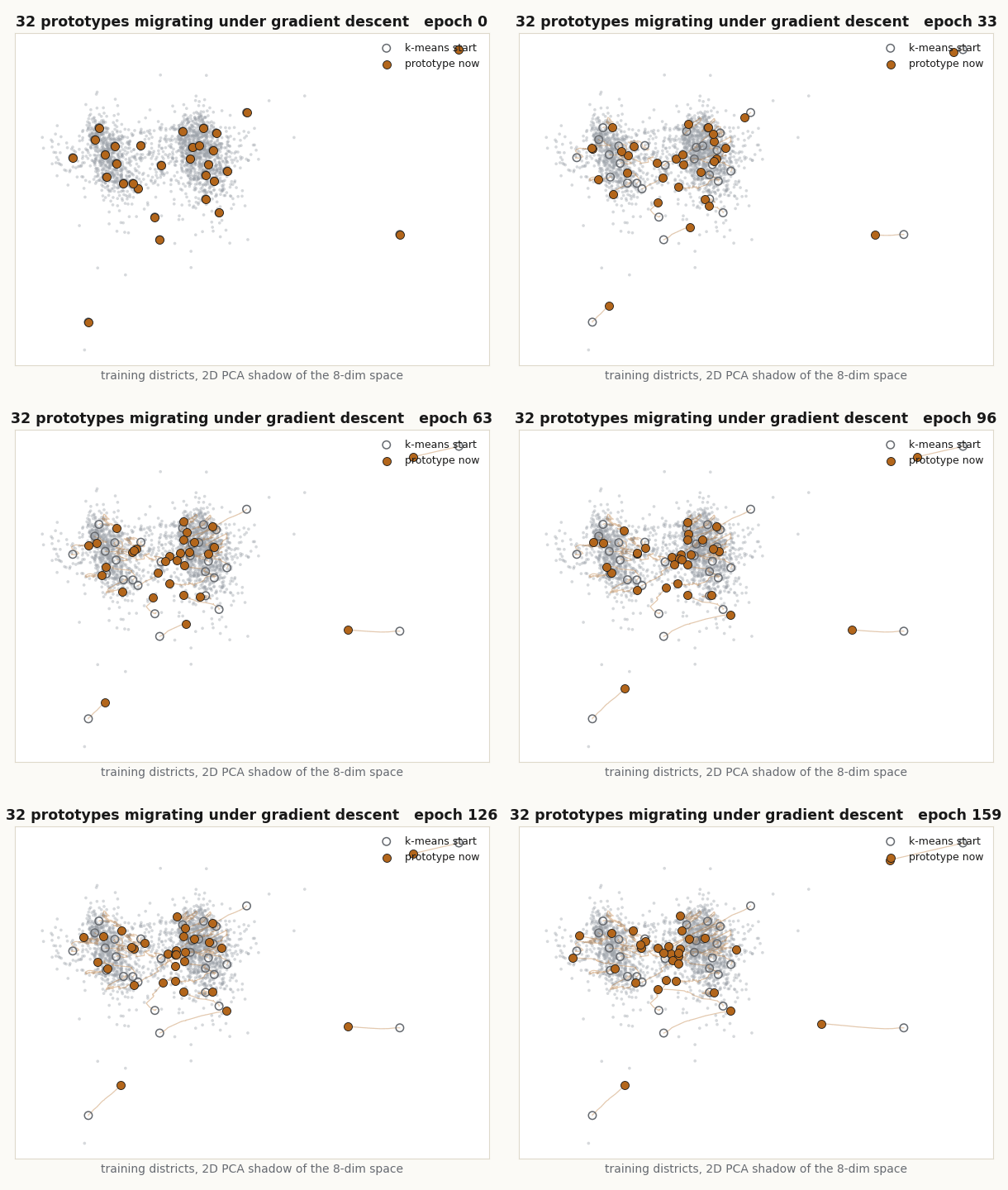
The protos argument decides what the centers mean on day one: they are k-means centroids of the training data, so every unit starts life as a summary of real districts rather than a random direction.

def kmeans_protos(X, K, seed):
    km = KMeans(n_clusters=K, n_init=4, random_state=seed).fit(X[:20000])
    return km.cluster_centers_.astype(np.float32)

Training is AdamW on minibatches of 256, and the loop earns its two extra moving parts. Gradient descent does not hand you a finished function the way a factorization does; it hands you a trajectory, and you have to decide which point on it to keep. The loop scores validation every epoch and snapshots whenever it improves:

model = YatNet(kmeans_protos(Xtr, K, seed), out_dim, rngs, eps=eps)
opt = nnx.Optimizer(model, optax.adamw(lr, weight_decay=1e-4), wrt=nnx.Param)

@nnx.jit
def step(m, o, xb, yb):
    l, grads = nnx.value_and_grad(loss_fn)(m, xb, yb)
    o.update(m, grads)
    return l

best = (np.inf, None, -1)
for ep in range(epochs):
    perm = rng.permutation(n)
    for i in range(0, n - batch + 1, batch):
        idx = perm[i:i + batch]
        step(model, opt, jnp.asarray(Xtr[idx]), jnp.asarray(ytr[idx]))
    vm = val_metric(model)
    if vm < best[0]:
        best = (vm, _snapshot(model), ep)
_restore(model, best[1])

The snapshot pair is two lines, and the copy in the first one is load-bearing:

def _snapshot(model):
    return jax.tree.map(lambda a: np.asarray(a).copy(), nnx.state(model, nnx.Param))

def _restore(model, snap):
    nnx.update(model, jax.tree.map(jnp.asarray, snap))

np.asarray on a JAX array can be a zero-copy view of device memory, and the jitted step is free to donate and overwrite old parameter buffers on its next call; without .copy() the “best epoch” you restore at the end can be whatever training later scribbled over it. The copy also moves the weights to host memory, so a long run does not pin one stale set of device buffers per improvement.

One fairness rule sits above the loop: no gradient model is ever run at a borrowed learning rate. Each configuration sweeps its own grid on validation and keeps the winner, which is the same role pick_lam_eps plays for the solve:

def sweep_lr(Xtr, ytr, Xva, yva, K, lrs, seed, epochs, batch, loss_kind, ...):
    best = (None, np.inf)
    for lr in lrs:
        vm, _, _ = train_yat_net(Xtr, ytr, Xva, yva, K, lr, seed, epochs, batch, loss_kind, ...)
        if vm < best[1]:
            best = (lr, vm)
    return best[0]

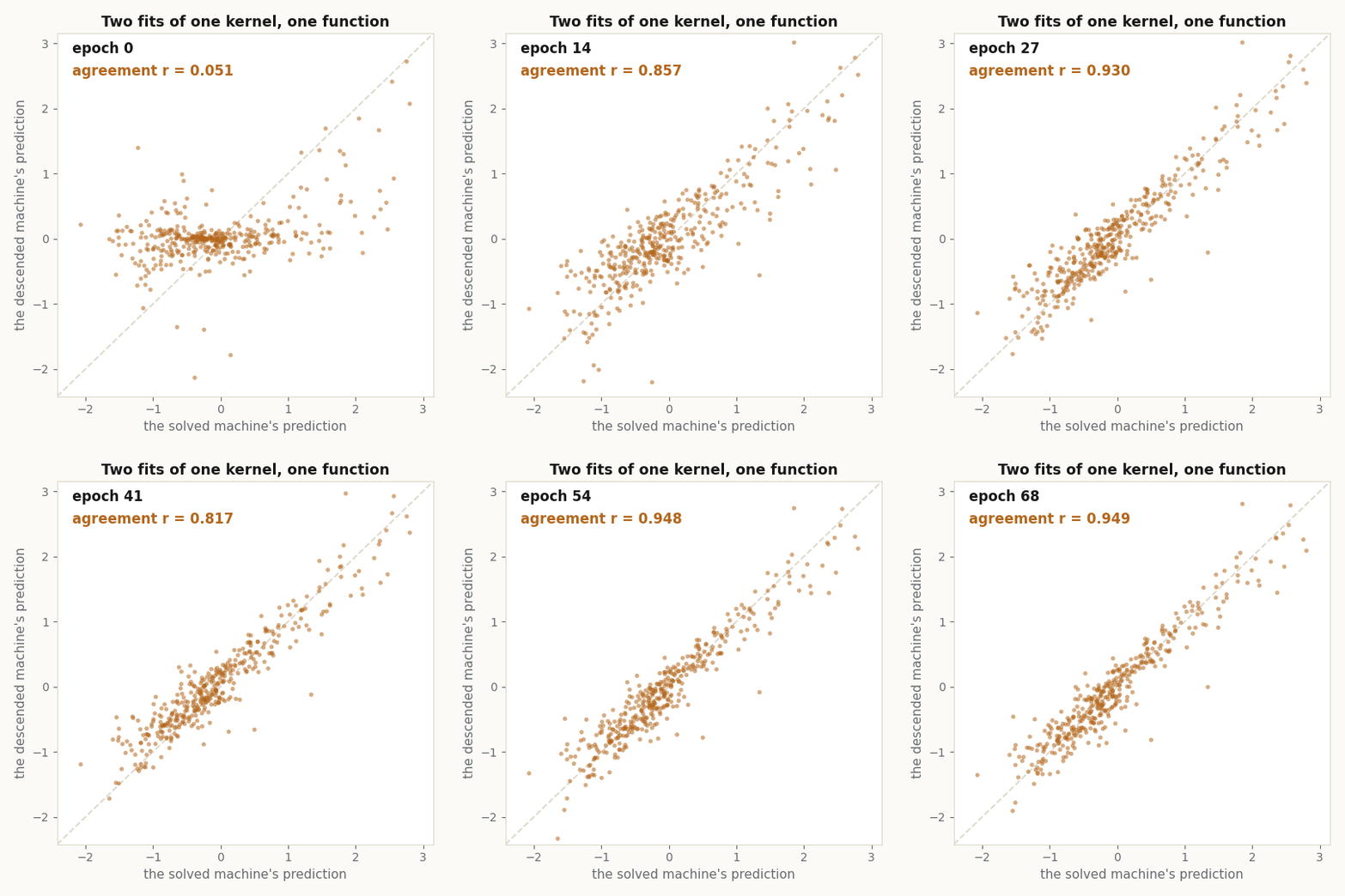
So both fits picked their hyperparameters on the same validation set, both carry eps = 10.22, and only the fitting procedure differs. At K = 64, over three seeds, the descended machine posts a test RMSE of 0.512 ± 0.002 against the solve’s 0.491, and the correlation between the two machines’ test predictions is r = 0.95. Here is that agreement forming, epoch by epoch, in the run’s own telemetry: 400 held-out predictions from the descending net plotted against the exact solve’s predictions for the same districts.

The control for the whole comparison is the escape route the field actually took. A random-features ridge (Rahimi and Recht, 2007) at the same parameter count, 320 dimensions, posts 0.506: the accuracy was never the issue. What it cannot do is name its centers, because it has none. The descended machine’s centers are points in district space, and you can watch them move under the gradient:

Timing the wall#

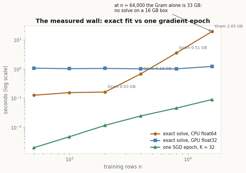
The explainer’s wall is a measured object, and the measurement is a plain loop: at each cohort size, time the CPU float64 solve, time a GPU float32 solve (Gram built and factorized on device), and time one SGD epoch of a 32-prototype net at batch 256, all on the same box.

for n in [500, 1000, 2000, 4000, 8000, 16000]:
    t0 = time.time()
    _, _ = solve_krr(Xn, yn, 1e-2)                     # CPU float64 exact solve
    cpu_s = time.time() - t0

    t0 = time.time()
    Kg = (dot * dot) / (jnp.maximum(sq, 0.0) + EPS) + 1e-2 * jnp.eye(n)
    L = jnp.linalg.cholesky(Kg)                        # GPU float32 exact solve
    al = jax.scipy.linalg.cho_solve((L, True), jnp.asarray(yn, jnp.float32))
    al.block_until_ready()
    gpu_s = time.time() - t0

    t0 = time.time()
    for i in range(0, n - 256 + 1, 256):               # one SGD epoch, K = 32
        step(model, opt, jnp.asarray(Xn[i:i + 256], jnp.float32),
             jnp.asarray(yn[i:i + 256], jnp.float32))
    jax.block_until_ready(model.a.value)
    sgd_epoch_s = time.time() - t0

The block_until_ready calls are what make the GPU numbers timings rather than dispatch latencies; JAX returns control before the work finishes, so an unblocked timer measures nothing. The measured rows: the CPU solve goes from 0.16 seconds at 2,000 rows to 19.6 at 16,000, a 122x cost for an 8x cohort. The GPU hides the cubic behind parallelism, a second flat across the whole range, but the float64 Gram is already 2.05 GB at 16,000 rows and clears the box’s 16 GB before 64,000, so the flat line just ends. One SGD epoch grows from 0.002 seconds at 500 rows to 0.090 at 16,000, linear the whole way, because nothing it holds is $n \times n$.

Minibatching through half a million rows#

Past the wall the two procedures stop being comparable, because only one of them still runs. Covertype is 511,012 training rows; the solve enters through subsamples, the descended net just iterates. The kernel is pinned once for everyone, eps picked on validation at n = 2,000 and shared by every solve size and every net, and then the same permute-and-slice loop from before eats the full training pool at batch 512:

perm = rng.permutation(n)                    # n = 511,012 on the last rung
for i in range(0, n - batch + 1, batch):
    idx = perm[i:i + batch]
    step(model, opt, jnp.asarray(Xtr[idx]), jnp.asarray(ytr[idx]))

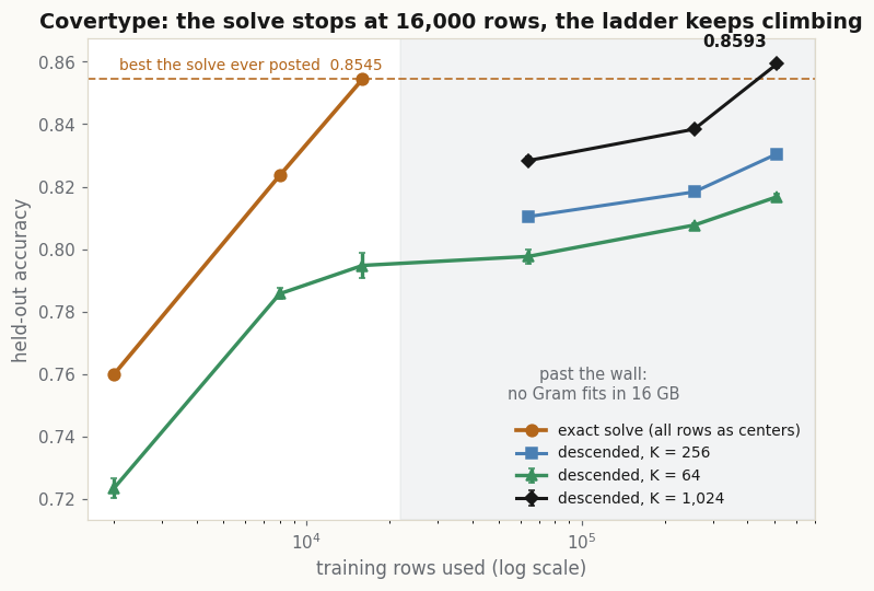
There is no other trick. The 64-prototype net holds 64 centers and 512 rows at a time no matter what n is, so “the whole dataset” is a wall-clock statement, not a memory one. The solve makes its subsamples count, 76.0% accuracy from 2,000 rows, 82.4% from 8,000, and 85.5% from 16,000, the stronger same-size fit at every rung, holding every row as a center. Then its Gram would need 33 GB and its column ends. The K = 64 net posts 79.5% at the same 16,000 rows, six points behind at 250x fewer parameters, and keeps going: 80.8% at 256,000 rows, 81.7% at all 511,012.

The second dial the solve never had is capacity. Since no Gram exists, K can scale with the data: 256 prototypes reach 83.0% on the full set, and 1,024 prototypes, given 20 epochs, reach 85.9% ± 0.1, past the best number the solve posted anywhere.

The head that trains its own eyes#

The last experiment is the one no amount of solver engineering answers, because it is not about cost. A solve consumes a fixed representation; a descendable head sits inside a network and shapes the representation beneath it. The composed model is two conv layers, a projection, and the same prototype head, the kernel arithmetic verbatim inside __call__:

class ConvYat(nnx.Module):
    """Two conv layers -> flatten -> Yat prototype head (K x 10)."""

    def __init__(self, K, rngs, feat_dim=64):
        self.c1 = nnx.Conv(1, 16, (3, 3), strides=2, rngs=rngs)
        self.c2 = nnx.Conv(16, 32, (3, 3), strides=2, rngs=rngs)
        self.proj = nnx.Linear(32 * 7 * 7, feat_dim, rngs=rngs)
        self.w = nnx.Param(0.5 * jax.random.normal(rngs.params(), (K, feat_dim)))
        self.b = nnx.Param(jnp.zeros((K,)))
        self.a = nnx.Param(0.01 * jax.random.normal(rngs.params(), (K, 10)))

    def features(self, x):
        h = jax.nn.relu(self.c1(x))
        h = jax.nn.relu(self.c2(h))
        return self.proj(h.reshape((h.shape[0], -1)))

    def __call__(self, x):
        f = self.features(x)
        dot = f @ self.w.value.T + self.b.value[None, :]
        sq = ((f[:, None, :] - self.w.value[None, :, :]) ** 2).sum(-1)
        return ((dot * dot) / (sq + EPS)) @ self.a.value

nnx.value_and_grad differentiates through the whole thing at once, head and trunk together, so the prototypes live in a feature space that is itself moving to make them work better. That is the loop the solve cannot join: its gradient would have nowhere to flow, because there is no gradient, only a factorization over whatever features it was handed.

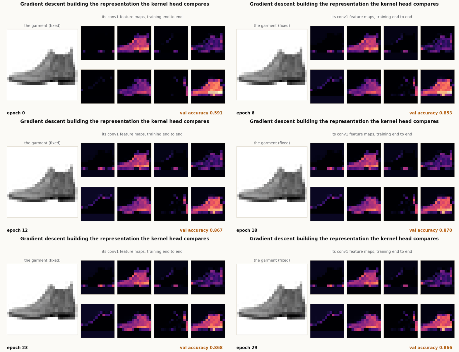
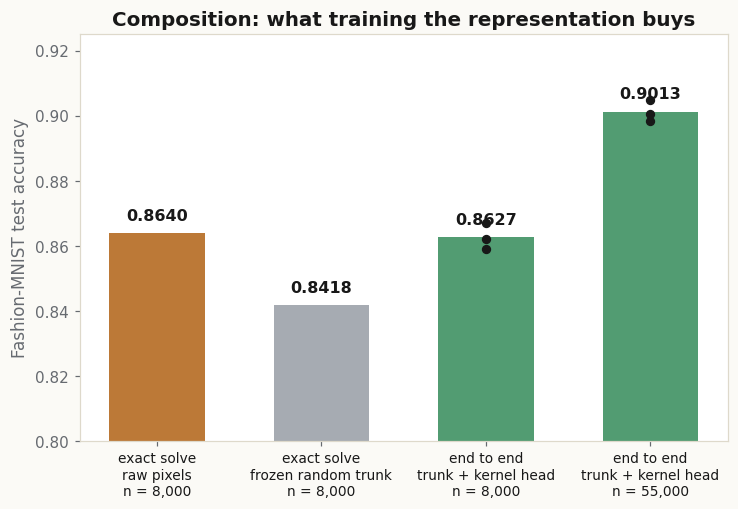
Three fits on Fashion-MNIST make the point. The exact solve on raw pixels, 8,000 rows, posts 86.4%. The same solve on the features of a frozen random ConvYat.features posts 84.2%, worse than the pixels it started from: an untrained representation is not a mild version of a trained one, it is a loss. The end-to-end model at the same 8,000 rows posts 86.3% ± 0.3, tying the raw solve, and at the full 55,000 rows, where a solve would need a 24 GB Gram, it takes 90.1% ± 0.3. And what the gradient actually buys is watchable. One test garment, held fixed; its first-layer feature maps, redrawn as the trunk trains under the kernel head:

That is the entire battery: one four-line kernel, a factorization that fits it exactly and must hold all of $n^2$ to do so, and a module that fits the same kernel by minibatch gradients and therefore scales, composes, and keeps its centers readable. The argument for why this matters, and the walls in order, live in the explainer.

@misc{bouhsine2026youdonthavetosolveakernelmachinejaxflaxnnx,
  author       = {Bouhsine, Taha},
  title        = {Solving It and Descending It, in JAX/Flax NNX},
  year         = {2026},
  month        = {jul},
  howpublished = {\url{https://tahabouhsine.com/blog/you-dont-have-to-solve-a-kernel-machine-jax-flax-nnx/}},
  note         = {Blog post, Records of the !mmortal Data Scientist}
}