Auditing Latent Space Geometry in JAX

The runnable companion to What Makes a Good Latent Space?. There I argued that a good latent space is a low-crosstalk codebook. Here we build the audit in JAX and render the same geometry as GIFs.

The point of the theory post was not “the Welch bound is cool.” The useful claim was operational:

Given a batch of embeddings, you should be able to tell whether the space is collapsing, whether it is using its dimensions, whether class means are moving toward a simplex, and whether an overloaded codebook is close to the Welch floor.

This post is that checklist. We will make five small JAX experiments, each with one question:

1. Are same-class points tightening?
2. Is the embedding using its dimensions?
3. When the classes fit, are the class codes becoming a simplex?
4. When they do not fit, how close is the worst crosstalk to Welch’s floor?
5. And can a plain optimizer even reach these targets, or is it luck?

The generator that made every GIF here lives in scripts/jax-welch-geometry/. The code blocks below are the core math stripped down to the pieces you would actually paste into a training loop.

The Shared Scaffolding#

Everything starts with two arrays:

import jax
import jax.numpy as jnp

# z: [n, d] embeddings
# y: [n] integer labels in {0, ..., c - 1}

Most of the geometry in the Welch post lives on the sphere, so first normalize rows:

def l2_normalize(x, eps=1e-8):
    return x / (jnp.linalg.norm(x, axis=-1, keepdims=True) + eps)

Then build the one matrix that explains almost everything:

def gram(z):
    z = l2_normalize(z)
    return z @ z.T

gram(z)[i, j] is a cosine. Bright off-diagonal blocks mean collapse or crosstalk. Blue off-diagonal entries mean negative correlation. A clean simplex has one repeated off-diagonal value. A good overloaded frame spreads absolute correlation evenly instead of letting one pair become the disaster pair.

For labeled embeddings, reduce examples to class codes:

def class_means(z, y, c):
    z = l2_normalize(z)
    one_hot = jax.nn.one_hot(y, c, dtype=z.dtype)
    counts = jnp.sum(one_hot, axis=0)[:, None]
    means = (one_hot.T @ z) / jnp.maximum(counts, 1.0)
    return l2_normalize(means)

That is the object we use for simplex and neural-collapse style audits:

m = class_means(z, y, c)
Gm = gram(m)

1. Collapse: Are Classes Tightening?#

Before asking whether the class means form a simplex, ask the simpler question: did each class become a point?

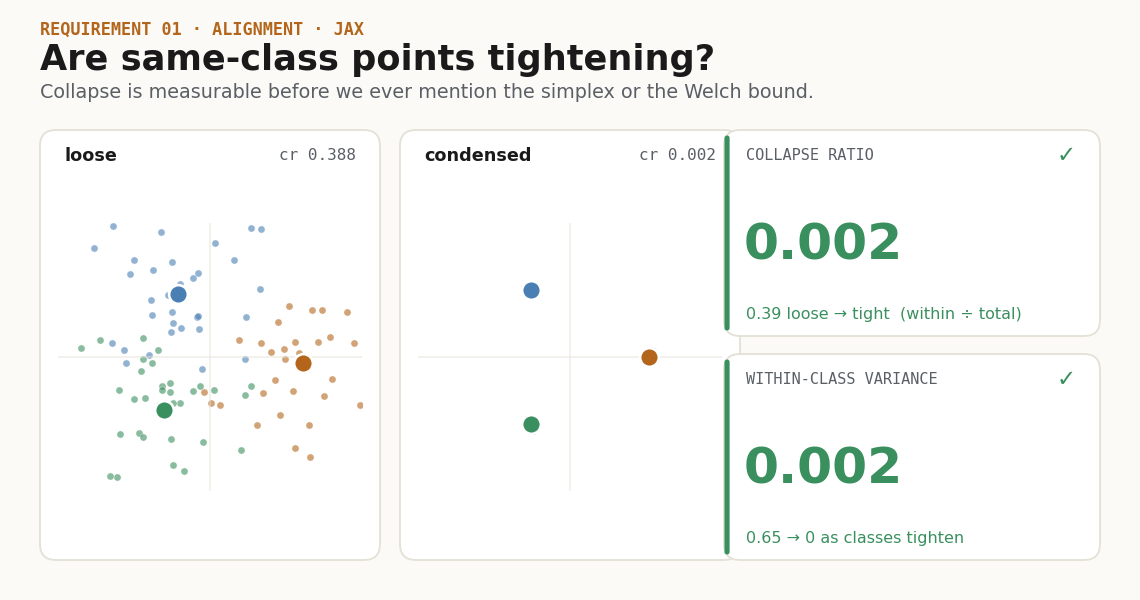
The direct metric is within-class variance:

def within_class_variance(z, y, c):
    z = l2_normalize(z)
    means = class_means(z, y, c)
    residual = z - means[y]
    return jnp.mean(jnp.sum(residual * residual, axis=-1))

For dashboards, I prefer a scale-free ratio: within-class scatter divided by total scatter.

def collapse_ratio(z, y, c, eps=1e-8):
    z = l2_normalize(z)
    means = class_means(z, y, c)
    global_mean = jnp.mean(z, axis=0, keepdims=True)
    within = jnp.mean(jnp.sum((z - means[y]) ** 2, axis=-1))
    total = jnp.mean(jnp.sum((z - global_mean) ** 2, axis=-1))
    return within / (total + eps)

This number answers the first audit question. It does not tell you whether the classes are arranged well; it only tells you whether each class is becoming a tight code. In neural collapse notation, this is the first thing that vanishes.

2. Rank: Is The Space Being Used?#

A model can make clusters look separated while secretly wasting dimensions. The next audit asks whether the embedding really occupies the axes available to it.

The covariance eigenvalues tell you where the energy went:

def covariance_eigs(z):
    z = z - jnp.mean(z, axis=0, keepdims=True)
    cov = (z.T @ z) / jnp.maximum(z.shape[0] - 1, 1)
    return jnp.linalg.eigvalsh(cov)

Convert those eigenvalues into an entropy-based effective rank:

def effective_rank(z, eps=1e-12):
    eigs = jnp.clip(covariance_eigs(z), 0.0)
    p = eigs / (jnp.sum(eigs) + eps)
    entropy = -jnp.sum(jnp.where(p > 0, p * jnp.log(p + eps), 0.0))
    return jnp.exp(entropy)

A round 2-D cloud gives roughly 2. A line gives roughly 1. In a 512-dimensional embedding, the exact value is less important than the trend: if this number is falling while your loss is improving, the model may be buying separation by destroying representational capacity.

3. Simplex: When The Class Codes Fit#

Now reduce each class to one normalized mean. If C centered class codes fit in the dimension, the simplex target is one repeated off-diagonal cosine:

In code, build the target Gram matrix:

def simplex_gram(c, dtype=jnp.float32):
    eye = jnp.eye(c, dtype=dtype)
    return eye + (1.0 - eye) * (-1.0 / (c - 1))

Then compare your class-mean Gram to that target:

def simplex_error(means):
    means = l2_normalize(means)
    c = means.shape[0]
    G = means @ means.T
    target = simplex_gram(c, G.dtype)
    return jnp.sqrt(jnp.mean((G - target) ** 2))

The GIF optimizes this error directly, just to make the target visible:

@jax.jit
def simplex_step(means, lr=0.04):
    loss, grad = jax.value_and_grad(lambda x: simplex_error(x) ** 2)(means)
    means = means - lr * grad
    return l2_normalize(means), loss

In a real training run you usually would not optimize simplex_error alone. You would log it. If it falls while the collapse ratio also falls, your class means are not merely separating; they are becoming the centered codebook the theory predicts.

4. Welch: When The Codes Do Not Fit#

The simplex is the friendly case. The crowded case is more common: too many codes, too few dimensions. Now the right question is not “can we make every pair orthogonal?” We cannot. The question is how low the worst crosstalk can go.

The worst absolute off-diagonal cosine is the coherence:

def coherence(x):
    x = l2_normalize(x)
    G = x @ x.T
    n = G.shape[0]
    off_diag = G - jnp.eye(n, dtype=G.dtype)
    return jnp.max(jnp.abs(off_diag))

The Welch floor is:

def welch_floor(c, d):
    c = jnp.asarray(c, dtype=jnp.float32)
    d = jnp.asarray(d, dtype=jnp.float32)
    return jnp.sqrt(
        jnp.maximum(c - d, 0.0) / (d * jnp.maximum(c - 1.0, 1.0))
    )

So the audit metric is:

def welch_gap(x):
    x = l2_normalize(x)
    c, d = x.shape
    return coherence(x) - welch_floor(c, d)

In the renderer I use a smooth approximation to the max so gradient descent can move the points:

def smooth_coherence_loss(x, beta=30.0):
    x = l2_normalize(x)
    G = x @ x.T
    n = G.shape[0]
    off_diag = jnp.where(jnp.eye(n, dtype=bool), -jnp.inf, jnp.abs(G))
    smooth_max = jax.nn.logsumexp(beta * off_diag) / beta

    # Keep the frame from lowering crosstalk by wasting dimensions.
    cov = (x.T @ x) / n
    tightness = jnp.sum((cov - jnp.eye(x.shape[1]) / x.shape[1]) ** 2)
    return smooth_max + 0.15 * tightness

That last tightness term matters. Without it, a toy optimizer can lower some pairwise terms while quietly wasting rank. The theory post kept saying the three requirements travel together: tight classes, low crosstalk, and full rank. The code has to respect the same bargain.

5. Reachability: Is The Geometry Even Findable?#

Every audit above assumes the optimizer can reach the target. It can — and not by luck. The frame potential $\sum_{i,j}\langle e_i, e_j\rangle^2$ has no bad local minima (Benedetto & Fickus, 2003), so every random start lands on the same floor $C^2/d - C$. The cleanest way to see that in JAX is to descend from many starts at once: a single vmap over a lax.scan descent.

Write the descent once as a pure lax.scan so it compiles into one fused loop and vmaps over a batch of seeds for free:

import optax

def frame_potential(x):
    return jnp.sum(gram(x) ** 2)               # Σ_ij ⟨e_i, e_j⟩²

def descent(x0, loss_fn, opt, steps):          # one projected-GD trajectory
    state = opt.init(x0)
    def body(carry, _):
        x, s = carry
        _, g = jax.value_and_grad(loss_fn)(x)
        u, s = opt.update(g, s, x)
        return (l2_normalize(optax.apply_updates(x, u)), s), x
    _, xs = jax.lax.scan(body, (x0, state), None, length=steps)
    return jnp.concatenate([x0[None], xs])

def run_many(key, c, d, n_seeds=6, steps=600):
    x0s = l2_normalize(jax.random.normal(key, (n_seeds, c, d)))
    one = lambda x0: descent(x0, frame_potential, optax.adam(0.05), steps)
    fp  = jax.vmap(jax.vmap(frame_potential))(jax.vmap(one)(x0s)) - c
    return fp                                  # every row → C²/d − C

The outer vmap runs six independent optimizations in parallel; the inner one audits every snapshot of every trajectory. (The - c drops the constant diagonal so the floor reads as the classic $C^2/d - C$.) They all converge to the same value, which is the practical payoff: you don’t have to be clever about initialization — the landscape does the work.

The Report Function#

For a real model, I would log one compact report every few hundred steps:

def latent_geometry_report(z, y, c):
    z = l2_normalize(z)
    means = class_means(z, y, c)

    return {
        "collapse_ratio": collapse_ratio(z, y, c),
        "within_class_variance": within_class_variance(z, y, c),
        "effective_rank": effective_rank(z),
        "class_simplex_error": simplex_error(means),
        "class_coherence": coherence(means),
        "class_welch_gap": welch_gap(means),
    }

At the logging boundary:

report = jax.device_get(latent_geometry_report(z, y, c))
report = {k: float(v) for k, v in report.items()}

The interpretation is straightforward:

• collapse_ratio down: classes are tightening.
• effective_rank high: the space is not wasting dimensions.
• class_simplex_error down: class means are becoming a simplex when they fit.
• class_coherence down: worst crosstalk is improving.
• class_welch_gap near zero: the overloaded codebook is close to the geometric floor.

The Gram matrix is the visual version of the same report:

G = jax.device_get(gram(class_means(z, y, c)))

Plot that matrix during training. If the off-diagonal entries become uniform, the story is happening.

Regenerate The GIFs#

The renderer lives in scripts/jax-welch-geometry/:

cd scripts/jax-welch-geometry
pip install -r requirements.txt
python generate.py

It validates each descent against theory, then writes five files:

• public/jax-welch/class-collapse.gif
• public/jax-welch/rank-collapse.gif
• public/jax-welch/simplex-descent.gif
• public/jax-welch/welch-descent.gif
• public/jax-welch/benign-landscape.gif

The important thing is that the pictures are not separate from the code. The same JAX arrays produce the points, Gram matrices, and metrics. The visual is just the audit report made visible.

@misc{bouhsine2026welchboundjaxanalysis,
  author       = {Bouhsine, Taha},
  title        = {Auditing Latent Space Geometry in JAX},
  year         = {2026},
  month        = {jun},
  howpublished = {\url{https://tahabouhsine.com/blog/welch-bound-jax-analysis/}},
  note         = {Blog post, Records of the !mmortal Data Scientist}
}