Latent on the Spectrum, in JAX
#ml#representation-learning#neural-collapse#simplex-etf#latent-space#spectral-embedding#kernel-methods#jax#implementation
The explainer reframed a codebook as the spectral embedding of a label-similarity kernel: diagonalise the kernel, keep its strongest modes, and the geometry follows the spectrum. This is the implementation companion: the classical-MDS embedding in JAX (with the square-root scaling done right), the flat→simplex and graded→horseshoe morph, kernel-target alignment, and the split of a trained representation into its prototype frame and its information spectrum, all as runnable jnp.linalg.eigh.
jnp.linalg.eigh.Everything here is plain JAX. The objects are tiny (a C × C label kernel, a handful of features) so the linear algebra is legible.
A codebook is the spectral embedding of a kernel
Given a target similarity S between classes, the best d-dimensional codebook whose Gram matrix approximates S is read straight off the spectrum. Ignoring the unit-norm step for a moment, the best rank-d Gram is , and a coordinate matrix that realises it is : the top-d eigenvectors scaled by the square roots of their eigenvalues. If we want cosine codes, we normalise afterward.
import jax
import jax.numpy as jnp


def spectral_codebook(S, d):
    """S: (C, C) symmetric label kernel -> C unit-norm codes in R^d."""
    w, V = jnp.linalg.eigh(S)                 # ascending eigenpairs
    w, V = w[::-1], V[:, ::-1]                # to descending
    coords = V[:, :d] * jnp.sqrt(jnp.clip(w[:d], 0.0, None))   # Lambda_d^{1/2} U_d^T : rows are codes
    return coords / (jnp.linalg.norm(coords, axis=1, keepdims=True) + 1e-9)
That single eigendecomposition is classical multidimensional scaling, the spectral fact behind kernel PCA and Laplacian eigenmaps. The reconstruction error of the rank-d codebook is exactly the tail of the spectrum:
def gram_error(S, d):
    w, V = jnp.linalg.eigh(S)
    w, V = jnp.clip(w[::-1], 0.0, None), V[:, ::-1]
    Shat = (V[:, :d] * w[:d]) @ V[:, :d].T
    return jnp.linalg.norm(Shat - S) / jnp.linalg.norm(S)     # falls as the kept modes capture more of S
The spectrum decides the geometry
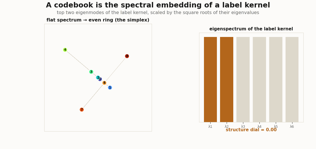
Three label kernels, three spectra, three shapes. The structureless kernel is flat and gives the even simplex; a block kernel is two-peaked and gives clusters; a graded kernel (similarity falling off with class distance) is the horseshoe of Diaconis, Goel & Holmes (2008).
C = 9
i = jnp.arange(C)

flat   = jnp.eye(C) - jnp.ones((C, C)) / C                       # structureless: the simplex
blocks = (i[:, None] // 3 == i[None, :] // 3).astype(jnp.float32)  # 3 superclasses of 3: clusters
graded = jnp.exp(-((i[:, None] - i[None, :]) / 2.2) ** 2)        # falls with class distance: the horseshoe

for name, S in [("flat", flat), ("blocks", blocks), ("graded", graded - graded.mean())]:
    codes = spectral_codebook(S, d=2)
    w = jnp.clip(jnp.linalg.eigh(S)[0][::-1], 0.0, None)
    print(name, "top-3 spectrum:", jnp.round(w[:3] / (w[0] + 1e-9), 2))
# flat   -> [1.   1.   1.  ]  (no preferred direction -> even ring)
# blocks -> [1.   ~.5  ~0  ]  (two dominant modes -> clusters)
# graded -> [1.   ~.7  ~.3 ]  (a smooth tail -> a curved 1-D manifold, the horseshoe)
The hero animation above is exactly this spectral_codebook(S, 2) evaluated along a dial from flat to graded, with each frame’s eigenvectors orthogonally aligned to the previous so the morph is smooth.
Kernel-target alignment
The reason this works is the old, exactly-right idea that the ideal embedding kernel is the label kernel (Cristianini et al., 2002). The match is one cosine between two Gram matrices:
def alignment(A, B):
    return jnp.sum(A * B) / (jnp.linalg.norm(A) * jnp.linalg.norm(B) + 1e-9)


codes = spectral_codebook(graded - graded.mean(), d=2)
gram = codes @ codes.T                                   # the codebook's own similarity
print(alignment(gram, graded - graded.mean()))           # high: the 2-D code already captures the kernel
Raise d and the alignment climbs toward 1 as the codebook is allowed to reproduce more of the kernel’s spectrum. The figure below sweeps that budget directly: for each d it rebuilds the rank-d Gram from the top eigenmodes and lays the reconstruction next to the target kernel, with alignment and gram_error charting the spend.
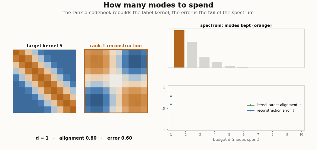
d the rank-d Gram matrix (the top d eigenmodes of the label kernel) is laid beside the target. As d grows the reconstruction sharpens back into the kernel, alignment climbs toward 1, and gram_error falls toward 0: the error you carry is exactly the tail of the spectrum you chose not to spend on.A handful of modes already recover most of a graded kernel, which is the whole reason a low-dimensional codebook works: the kernel’s mass lives in its top eigenvalues, and the rest is a tail you can drop.
The prototype frame and the information spectrum
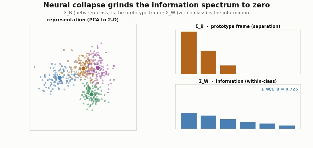
Now switch objects: from the target label kernel to a trained representation. Split a feature matrix into between-class and within-class covariance. The between-class part has rank at most C-1 and spans the prototypes: it is the separation channel, the codebook. The within-class part is everything else: the gradations the codebook does not carry, the information.
def class_covariances(Z, y, C):
    mu = jnp.stack([Z[y == c].mean(0) for c in range(C)])
    g, N = Z.mean(0), Z.shape[0]
    SB = sum((y == c).sum() * jnp.outer(mu[c] - g, mu[c] - g) for c in range(C)) / N
    SW = jnp.mean(jax.vmap(lambda z, c: jnp.outer(z - mu[c], z - mu[c]))(Z, y), 0)
    return SB, SW


SB, SW = class_covariances(Z, y, C)
eig_B = jnp.clip(jnp.linalg.eigvalsh(SB)[::-1], 0.0, None)   # <= C-1 nonzero: the prototype frame
eig_W = jnp.clip(jnp.linalg.eigvalsh(SW)[::-1], 0.0, None)   # the information tail
print("nonzero prototype modes:", int((eig_B > 1e-6 * eig_B[0]).sum()), "  (C-1 =", C - 1, ")")
The split is clean only when the between-class variance dominates, as it does near neural collapse; with large within-class variance the two regimes overlap. The figure below trains a small encoder with cross-entropy and watches it happen: sharpens into a C-1-mode simplex frame while the spectrum is ground toward zero (Papyan, Han & Donoho, 2020).
Dark knowledge is the coefficients
The explainer’s last move: the information that survives lives between the prototypes, as the soft mixture a feature makes over them, the dark knowledge a teacher distils (Hinton et al., 2015). In this frame view it is a coefficient vector, a soft assignment over the prototype frame:
def soft_assignment(z, prototypes, tau=0.1):
    """z: (..., d) feature; prototypes: (C, d). Returns coefficients over the codebook."""
    return jax.nn.softmax((z @ prototypes.T) / tau, axis=-1)


a = soft_assignment(z, mu)        # e.g. [0.70, 0.27, 0.02, 0.01]: "mostly cat, a bit dog"
Sharpen tau → 0 and the vector collapses to one-hot, and the relation between classes is erased, exactly the effect label smoothing and a low temperature have. The information is the off-one-hot mass. On a graded codebook the point is visible in the geometry: a feature near class k lends its mass to k’s neighbours on the horseshoe, so the assignment encodes which classes are similar, and cooling the temperature burns that structure away.
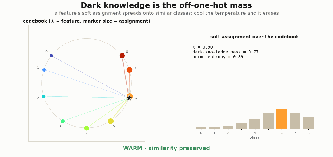
soft_assignment is shown as marker sizes (left) and bars (right). Warm: the mass spreads onto the geometric neighbours (5, 7, 8), encoding class similarity, with a high dark-knowledge mass and entropy. Cool the temperature and it collapses to a one-hot spike on class 6: the relation between classes is erased and the dark-knowledge mass goes to 0.Rendering the GIFs
All four animations are generated with Python, JAX, and matplotlib: the linear algebra in JAX, the drawing in matplotlib:
python scripts/render_spectral_codebook_gif.py     # flat -> simplex -> horseshoe morph
python scripts/render_mds_reconstruction_gif.py    # rank-d Gram rebuild, alignment up / error down
python scripts/render_information_collapse_gif.py  # neural collapse of the Σ_W spectrum
python scripts/render_dark_knowledge_gif.py        # temperature sweep, soft assignment -> one-hot
The first sweeps a label kernel from flat to graded, recomputing spectral_codebook(S, 2) and the eigenspectrum each frame (with Procrustes alignment between frames so the morph is smooth). The second sweeps the budget d, rebuilding the rank-d Gram and recomputing alignment and gram_error. The third trains a small encoder and recomputes class_covariances each frame. The fourth fixes a graded codebook and sweeps the softmax temperature, recomputing soft_assignment each frame. None is a benchmark; they are visual audits of the spectrum.
What this leaves out
A production embedding would use far more classes, real data, and a deep encoder, and the label kernel would be estimated rather than handed to you. The point this companion keeps is the one the explainer named: a codebook is a spectrum, the prototypes are its top, and the information is the tail.
References: classical MDS / kernel-target alignment from Cristianini et al. (2002); the horseshoe from Diaconis, Goel & Holmes (2008); neural collapse from Papyan et al. (2020); dark knowledge from Hinton et al. (2015); the Welch bound from Welch (1974).
Cite as
Bouhsine, T. (). Latent on the Spectrum, in JAX. Records of the !mmortal Data Scientist. https://tahabouhsine.com/blog/latent-on-the-spectrum-jax/
BibTeX
@misc{bouhsine2026latentonthespectrumjax,
  author       = {Bouhsine, Taha},
  title        = {Latent on the Spectrum, in JAX},
  year         = {2026},
  month        = {jun},
  howpublished = {\url{https://tahabouhsine.com/blog/latent-on-the-spectrum-jax/}},
  note         = {Blog post, Records of the !mmortal Data Scientist}
}References
- (1974). Lower Bounds on the Maximum Cross Correlation of Signals. IEEE Transactions on Information Theory 20(3).doi:10.1109/TIT.1974.1055219
- (2002). On Kernel-Target Alignment. NIPS 2001.
- (2008). Horseshoes in Multidimensional Scaling and Local Kernel Methods. Annals of Applied Statistics 2(3).arXiv:0811.1477
- (2020). Prevalence of Neural Collapse During the Terminal Phase of Deep Learning Training. PNAS 117(40).arXiv:2008.08186
- (2015). Distilling the Knowledge in a Neural Network. arXiv:1503.02531