The Price List, in JAX/Flax NNX
#ml#kernels#rkhs#representer-theorem#regularization#generalization#eigenvalues#jax#flax#nnx#implementation
Part 5 of 5Weights in Kernel Space
The explainer argued that the RKHS norm is a price list: every kernel splits into modes priced by eigenvalues, a weight pays for the modes it uses, and regularization is just tightening the budget. This is the implementation. A Gaussian kernel in a few lines of JAX, the representer solve , the bill , the effective dimension read off the Gram spectrum, and a sweep over that draws the generalization U-curve. There is no gradient descent anywhere: kernel ridge on a small dataset is one linear solve plus one eigendecomposition. Every number below is from that run; the script is scripts/regularization_pricelist.py and the GIFs are scripts/render_reg_gifs.py.
The kernel and the solve
Where is the budget in the code? It is a single scalar in a single solve. The whole machine is a Gaussian kernel, its Gram matrix on the training points, and the ridge system . That system is the representer weight solved in one shot, and the only thing does is inflate the diagonal, which shrinks every coefficient at once.
import jax, jax.numpy as jnp

SIG = 0.45

@jax.jit
def gram(A, B):                                       # k(xᵢ, yⱼ) for every pair
    d2 = ((A[:, None, :] - B[None, :, :]) ** 2).sum(-1)
    return jnp.exp(-d2 / (2 * SIG ** 2))

def kernel_ridge(K, y, lam):                          # the representer solve, no descent
    return jnp.linalg.solve(K + lam * jnp.eye(len(K)), y)
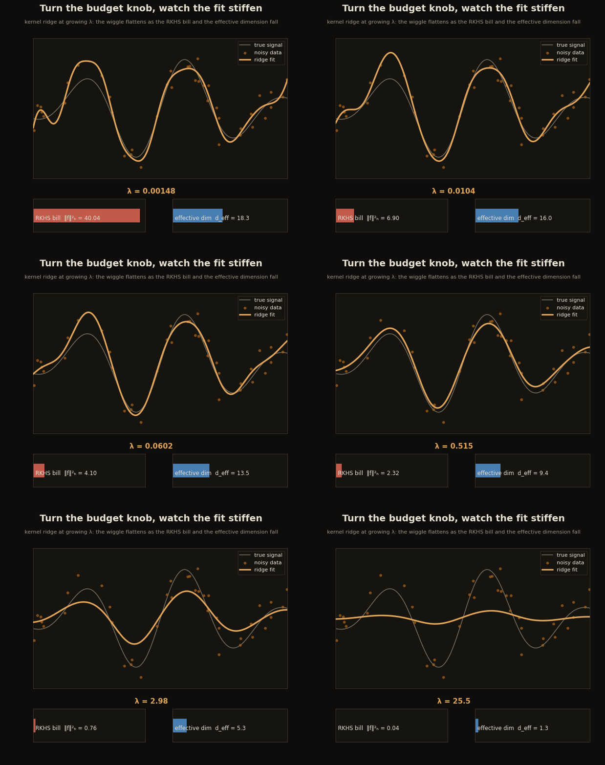
The vector alpha that comes back is the weight, one charge per training point. Turn up and the whole vector deflates. On a 1-D regression toy (a noisy damped sine, 40 training points, a clean test grid of 400) that deflation is the fit going from ferocious wiggle to smooth, while two readouts fall with it: the RKHS bill and the effective dimension.
scripts/render_reg_gifs.py.The bill you pay for the weight
So what is the bill, exactly? The explainer’s whole argument is that “expensive” is a real number you can compute from nothing but the kernel: the squared RKHS norm of the solution is . It is one line, and it is the quantity is capping.
def rkhs_norm_sq(K, alpha):                           # ‖f‖²_H, the bill
    return float(alpha @ (K @ alpha))
That single number falls monotonically as tightens: the ferocious fit spends , the fit at the generalization sweet spot spends , and the over-tight fit spends almost nothing, . The bill is the budget spent, and the knob is literally the spending limit.
The price list: eigenvalues and the effective dimension
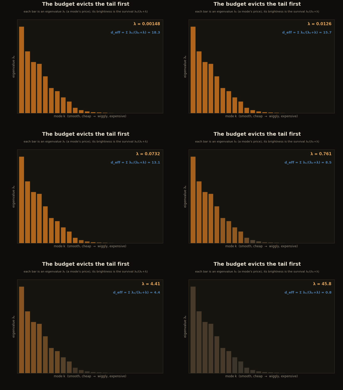
But a single cap does not tell you which modes get cut. That is set by the eigenvalues of the Gram matrix, the posted prices, and one symmetric eigendecomposition hands you the whole list.
eigs = jnp.linalg.eigvalsh(K)[::-1]                   # the price list, descending

def eff_dim(eigs, lam):                               # modes that survive the budget
    return float(jnp.sum(eigs / (eigs + lam)))
Each mode contributes , a survival weight that is near when the mode is cheap relative to the budget and near when it is not. Summed, that is the effective dimension: the number of directions the weight is actually allowed to use. Watch the budget evict the tail first, the expensive high-frequency modes going dark before the cheap smooth ones even dim.
scripts/render_reg_gifs.py.The points-to-modes bridge
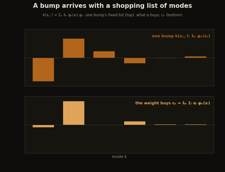
The representer weight is written one point at a time; the price list charges one mode at a time. The two currencies exchange through the Gram eigenvectors. Writing , the discrete Mercer modes are , a bump’s shopping list is , and buying the combination purchases mode in amount .
evals, U = jnp.linalg.eigh(K)                         # K = Σ λₖ uₖ uₖᵀ
c = evals * (U.T @ alpha)                             # cₖ = λₖ (uₖ · α), the mode purchase
bill_modes  = float(jnp.sum(c ** 2 / evals))          # Σ cₖ²/λₖ  ...
bill_direct = float(alpha @ (K @ alpha))              # ... equals αᵀKα, exactly
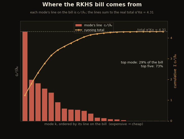
The two bills agree to machine precision in the run: priced by modes, priced by points, a relative error of . It is one weight, quoted in two currencies. A bump does not walk in empty-handed: it carries a fixed shopping list of modes, and only chooses how many copies of each list to buy.
scripts/render_reg_gifs.py.Once the weight is priced by modes, the bill breaks down line by line: each mode adds to the RKHS norm, the expensive lines dominating, up to the same real total .
scripts/render_reg_gifs.py.The shrink is graded, never zero
The explainer drew one distinction and this companion keeps it: kernel ridge is not a support-vector machine. It solves , and unlike a hinge loss it never sets a coefficient exactly to zero. Tightening shrinks every smoothly, just at very different rates, so what you get is a graded hierarchy, not a hard roster of survivors. On the six-point, two-class miniature from the explainer, the coefficients start at and, at the tightest budget, all sink toward a common floor with a minimum of , still strictly positive.
for lam in lambdas:                                   # the sweep, one solve each
    alpha = kernel_ridge(K, y, lam)
    abs_alpha = jnp.abs(alpha)                         # all shrink, none hit zero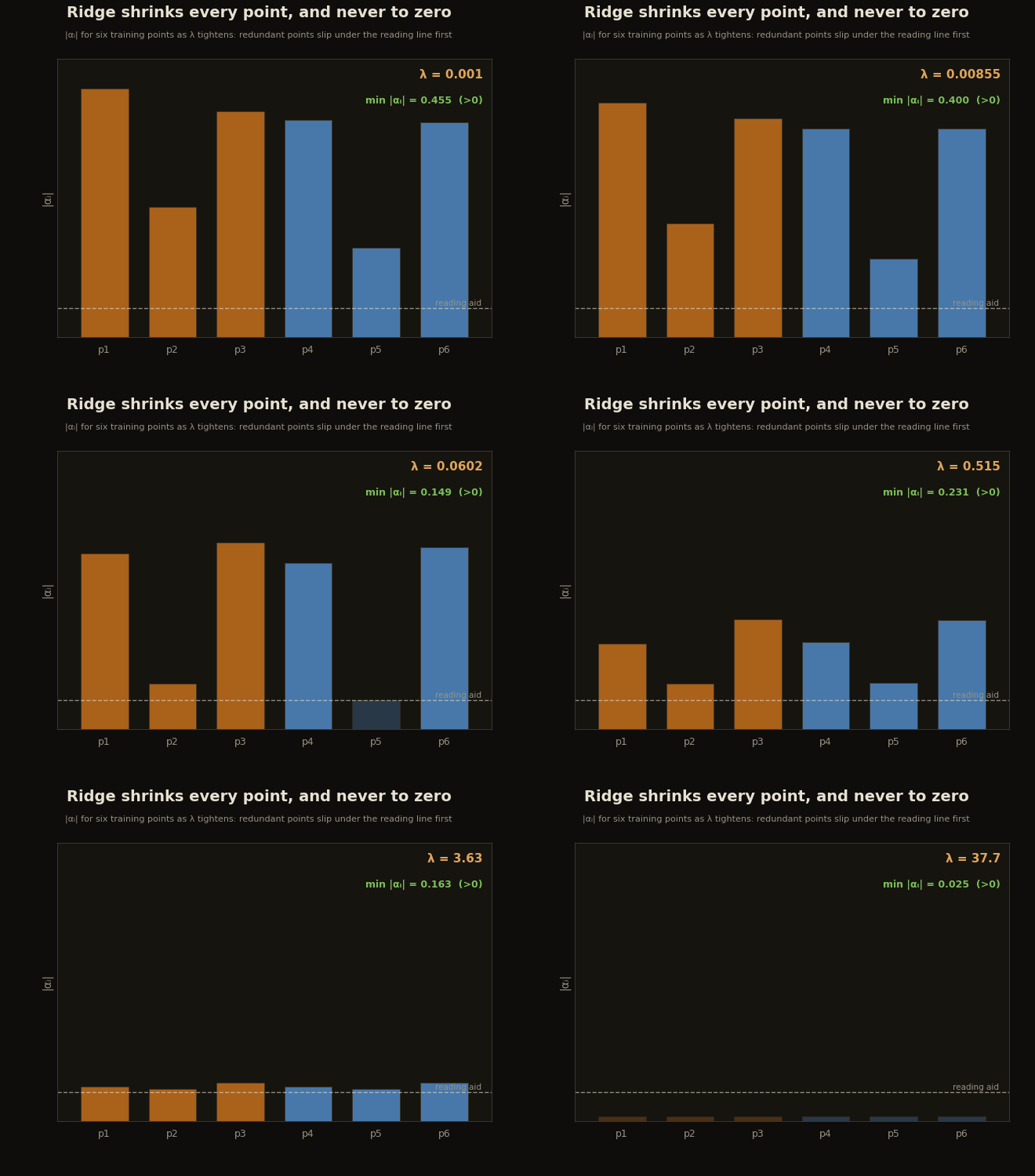
scripts/render_reg_gifs.py.Why smooth generalizes: the sweep
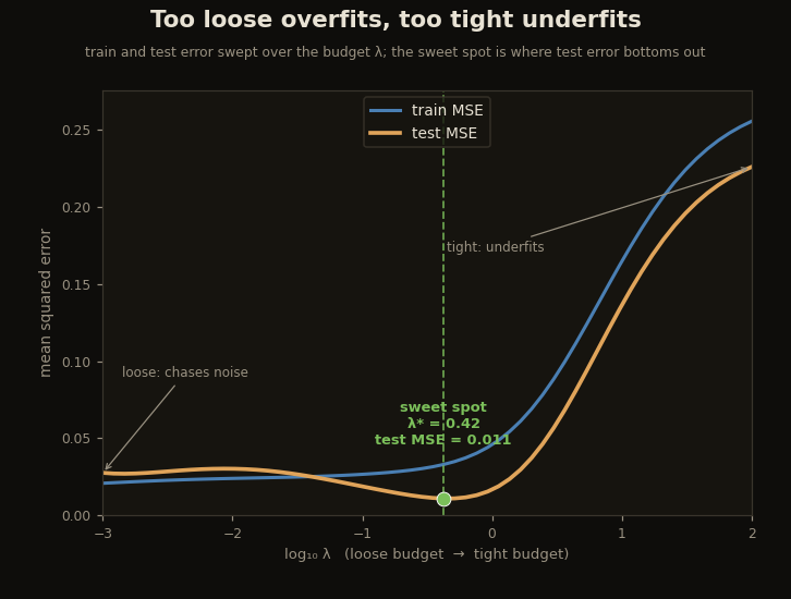
None of this matters unless the tight budget actually generalizes better, so the last thing the run does is sweep across five orders of magnitude and measure train and test error at each. That sweep draws the U-curve, and it is the whole point of the post.
for lam in lambdas:
    alpha = kernel_ridge(K_train, y_train, lam)
    train_mse = jnp.mean((K_train @ alpha - y_train) ** 2)
    test_mse  = jnp.mean((K_test  @ alpha - y_test)  ** 2)   # K_test is test-to-train
At a loose budget the fit chases the noise and test error sits above train (test MSE ); at an over-tight budget it underfits and test error explodes (test MSE ); in between, at , test error bottoms out at , where the effective dimension is of the available modes. The sweet spot is not where the training error is lowest; it is where the price list has capped the capacity to just what the signal needs.
scripts/render_reg_gifs.py.That is the price list made runnable. One kernel, one solve, one scalar budget. The eigenvalues post the prices, the effective dimension counts what the budget can afford, the bill is , and the U-curve is the payoff: the weight generalizes not because it is a free combination of the data but because it is a combination the price list can afford.
The representer theorem is Schölkopf, Herbrich and Smola (2001); the eigenvalue-price-list framing is standard RKHS theory in Steinwart and Christmann (2008); the effective-dimension complexity bound is Bartlett and Mendelson (2002); the input-space-center kernel this series builds on is Bouhsine (2026). The conceptual companion is Why Regularization Is a Price List.
Cite as
Bouhsine, T. (). The Price List, in JAX/Flax NNX. Records of the !mmortal Data Scientist. https://tahabouhsine.com/blog/regularization-is-a-price-list-jax-flax-nnx/
BibTeX
@misc{bouhsine2026regularizationisapricelistjaxflaxnnx,
  author       = {Bouhsine, Taha},
  title        = {The Price List, in JAX/Flax NNX},
  year         = {2026},
  month        = {jul},
  howpublished = {\url{https://tahabouhsine.com/blog/regularization-is-a-price-list-jax-flax-nnx/}},
  note         = {Blog post, Records of the !mmortal Data Scientist}
}References
- (2001). A Generalized Representer Theorem. COLT 2001.
- (2008). Support Vector Machines. Springer.
- (2002). Rademacher and Gaussian Complexities: Risk Bounds and Structural Results. JMLR.
- (2026). A Universal Reproducing Kernel Hilbert Space from Polynomial Alignment and IMQ Distance. arXiv:2605.03262