A White-Box DeepSurv, in JAX/Flax NNX
#survival-analysis#deepsurv#cox#kernels#interpretability#yat#healthcare-ml#jax#flax#nnx#implementation
Part 8 of 12The Prototype Network
- 1What a Finite Kernel Buys an MLP
- 2Your Neuron Is a Direction. It Should Be a Picture.
- 3Your Network Is a List of Pictures. You Can Edit It.
- 4You Only Have to Train the Features
- 5You Don't Even Have to Train the Features
- 6How Far Down Can You Build?
- 7When 80% Should Mean 80%
- 8A Risk Model That Names Its Reasonsthis post's explainer
- 9The White-Box Survival Model on Trial
- 10Your Network Is a Stack of Layers. It Could Be a Fixed Point.
- 11Edit One Operator, Edit Every Depth
- 12One Kernel, Fitted Twice
The explainer built a survival model whose risk score decomposes into the prototype patients it resembles, and matched a standard DeepSurv on the concordance index while doing it. This is the implementation: the Cox partial-likelihood loss, both models in Flax NNX, the concordance evaluation, and the interpretability and editing code, each a short block. Every number below is from a real run; the script is scripts/yat_deepsurv.py, on the METABRIC breast-cancer cohort, and this is a research illustration, not a clinical tool.
The loss is the whole model
A DeepSurv is defined by its loss, not its architecture: any network that outputs one scalar log-risk per patient can be trained by the Cox partial likelihood, and the rest is a choice of trunk. So the loss comes first. At each observed death, the model should have scored the patient who died above everyone still at risk at that moment. Sort patients by descending time and the risk set of an event becomes a running prefix, so the log of the risk-set sum is a cumulative logsumexp from the top.
import jax, jax.numpy as jnp

def cox_ph_loss(logrisk, times, events):
    """Negative Cox partial log-likelihood (Breslow ties)."""
    order = jnp.argsort(-times)                 # descending time
    h = logrisk[order]; ev = events[order]
    m = jnp.max(h)                              # stabilize the logsumexp
    log_cum = m + jnp.log(jnp.cumsum(jnp.exp(h - m)) + 1e-12)  # log Σ_{risk set} e^h
    return -jnp.sum((h - log_cum) * ev) / (jnp.sum(ev) + 1e-8)
Only observed events (ev == 1) contribute a term, but censored patients are not discarded: they sit inside the risk-set sums of every death that preceded their censoring time. That is how the partial likelihood uses a patient you only watched for a while without inventing a death date for them.
Two trunks, one output
With the loss fixed, the two models differ by one attribute. The standard DeepSurv is a ReLU MLP; the Yat DeepSurv is a bank of prototype kernels. Both map covariates to one log-risk.
from flax import nnx

class YatLayer(nnx.Module):
    def __init__(self, d_in, k, *, rngs, Winit, b0=1.0, eps0=1.0):
        self.W = nnx.Param(jnp.asarray(Winit))                 # [K, d] prototype patients
        self.log_b = nnx.Param(jnp.full((), jnp.log(jnp.expm1(b0))))
        self.log_eps = nnx.Param(jnp.full((), jnp.log(jnp.expm1(eps0))))

    def __call__(self, x):
        b, eps = jax.nn.softplus(self.log_b.value), jax.nn.softplus(self.log_eps.value)
        dot = x @ self.W.value.T
        d2 = jnp.sum(x**2, -1, keepdims=True) + jnp.sum(self.W.value**2, -1) - 2 * dot
        return (dot + b)**2 / (d2 + eps)                       # [n, K] kernel activations

class YatSurv(nnx.Module):
    """Yat DeepSurv: prototype-kernel trunk -> scalar log-risk h(x) = Σ a_u φ_u(x)."""
    def __init__(self, d_in, k, *, rngs, Winit):
        self.yat = YatLayer(d_in, k, rngs=rngs, Winit=Winit)
        self.read = nnx.Linear(k, 1, use_bias=False, rngs=rngs)  # the readout weights a_u

    def features(self, x): return self.yat(x)
    def __call__(self, x):  return self.read(self.yat(x))[:, 0]

class MLPSurv(nnx.Module):
    """Standard DeepSurv: ReLU MLP -> scalar log-risk."""
    def __init__(self, d_in, k, *, rngs):
        self.l1 = nnx.Linear(d_in, k, rngs=rngs)
        self.l2 = nnx.Linear(k, k, rngs=rngs)
        self.out = nnx.Linear(k, 1, use_bias=False, rngs=rngs)
    def __call__(self, x):
        h = jax.nn.relu(self.l2(jax.nn.relu(self.l1(x))))
        return self.out(h)[:, 0]
The Yat trunk’s prototypes are seeded from k-means centroids on the training patients, so the model starts legible: each unit is already a plausible patient before a single gradient step. Training is full-batch, because the risk set is global (every patient’s loss term looks at every later patient), which makes full-batch the natural and standard choice at this data size.
import optax

@nnx.jit
def train_step(model, opt, xb, tb, eb):
    def loss_fn(m): return cox_ph_loss(m(xb), tb, eb)
    loss, grads = nnx.value_and_grad(loss_fn)(model)
    opt.update(model, grads)
    return loss

def train(model, X, t, e, epochs=400, lr=3e-3, wd=1e-4):
    opt = nnx.Optimizer(model, optax.adamw(lr, weight_decay=wd), wrt=nnx.Param)
    Xj, tj, ej = jnp.asarray(X), jnp.asarray(t), jnp.asarray(e)
    for _ in range(epochs):
        train_step(model, opt, Xj, tj, ej)
    return model
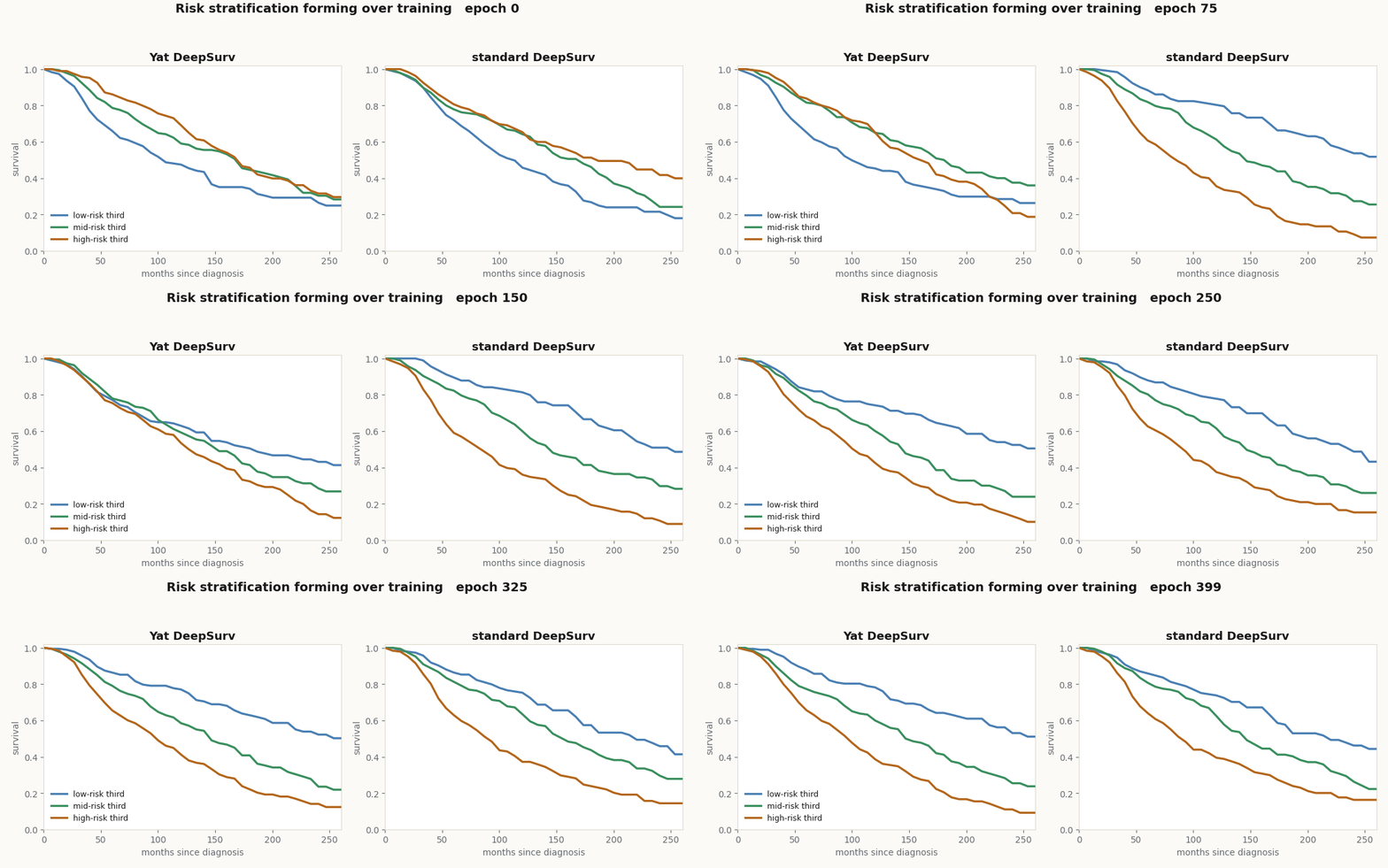
The stratification below is what those 400 epochs buy: split the held-out patients into risk tertiles by the model’s log-risk, and draw each tertile’s Kaplan-Meier curve as training proceeds. Both models pull the three curves apart; the Yat model’s separation is at least as clean.
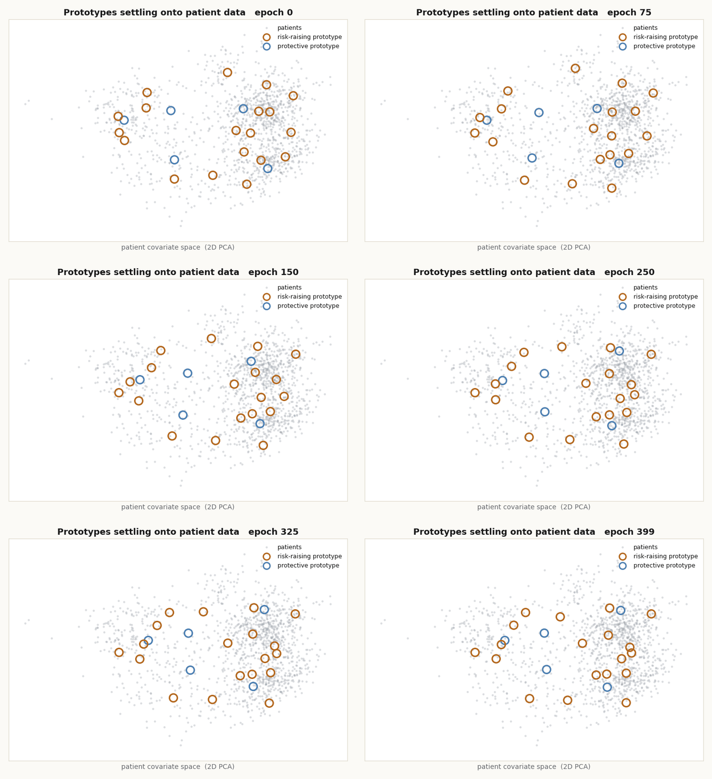
scripts/yat_deepsurv.py.As the prototypes train, they migrate off their k-means seeds and settle onto the structure the partial likelihood cares about. Because a prototype is a point in patient space, that migration is literally visible: project the covariates to two dimensions and watch the prototype rings drift across the patient cloud.
W parameters at each logged epoch, no synthetic path. From scripts/yat_deepsurv.py.Concordance: does it rank?
The scoreboard for a survival model is Harrell’s concordance index: over all pairs of patients whose ordering is known (one died before the other was censored), the fraction the model ranks correctly. Chance is 0.5. We use scikit-survival’s estimator so the censoring bookkeeping is standard.
from sksurv.metrics import concordance_index_censored

def cindex(model, X, t, e):
    risk = np.asarray(model(jnp.asarray(X)))          # higher = earlier event
    return concordance_index_censored(e.astype(bool), t, risk)[0]
Trained at matched capacity (24 hidden units) across three seeds, the two trunks tie on discrimination and the Yat trunk edges ahead on the probabilistic scores:
| metric | Yat DeepSurv | standard DeepSurv |
|---|---|---|
| C-index | 0.627 ± 0.033 | 0.623 ± 0.011 |
| time-dependent AUC | 0.653 ± 0.049 | 0.652 ± 0.016 |
| integrated Brier (lower better) | 0.199 ± 0.014 | 0.225 ± 0.008 |
| Cox partial NLL (lower better) | 5.64 ± 0.19 | 6.84 ± 0.40 |
Attribution is a subtraction
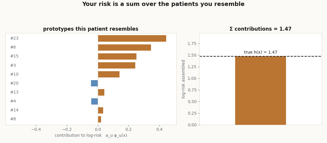
The point of the Yat trunk is that its log-risk has parts. Because h(x) = read(yat(x)) is linear in the kernel activations, the exact per-prototype contribution is an element-wise product, no gradients, no approximation.
phi = np.asarray(model.yat(jnp.asarray(X)))           # [n, K] kernel activations
a   = np.asarray(model.read.kernel.value)[:, 0]       # [K] readout weights
contrib = phi * a[None, :]                             # [n, K] signed contributions
assert np.allclose(contrib.sum(1), np.asarray(model(jnp.asarray(X))), atol=1e-3)
The contributions sum back to the log-risk to within on the held-out set, so a patient’s score is genuinely the sum of named prototype terms.
scripts/yat_deepsurv.py.Cohort deletion is a masked readout
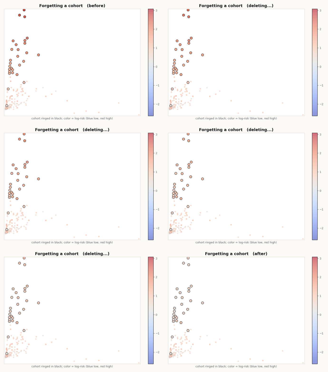
To forget a cohort, find the prototype it is built around and zero that readout weight. The change to every patient is the exact closed form for the deleted prototype , computable and auditable per patient.
assign = phi.argmax(1)                                # each patient's nearest prototype
# pick the prototype whose contribution mass is most concentrated on its own cohort
share = [np.abs(contrib[assign == u, u]).sum() / (np.abs(contrib[:, u]).sum() + 1e-9)
         for u in range(K)]
u = int(np.argmax([s if (assign == i).sum() >= 8 else -1 for i, s in enumerate(share)]))
cohort = assign == u                                  # the patients built around prototype u

a_edit = a.copy(); a_edit[u] = 0.0                    # zero that readout weight, no retraining
risk_before = (phi * a[None, :]).sum(1)
risk_after  = (phi * a_edit[None, :]).sum(1)
delta = risk_after - risk_before                      # = -a[u] * phi[:, u], exact per patient
On dense clinical covariates the deletion is not local the way it was on sparse images: every patient activates every prototype a little, so everyone moves by some exact amount. But the movement concentrates where the kernel says it should. Deleting prototype #12 (69% of its contribution mass on its own 28-patient cohort), the cohort shifts by 1.02 in log-risk on average; everyone else by 0.024, with 89% moving less than 0.05. The change to any patient is exactly their own resemblance to #12, a closed form you can show a regulator.
scripts/yat_deepsurv.py.Abstention is a max
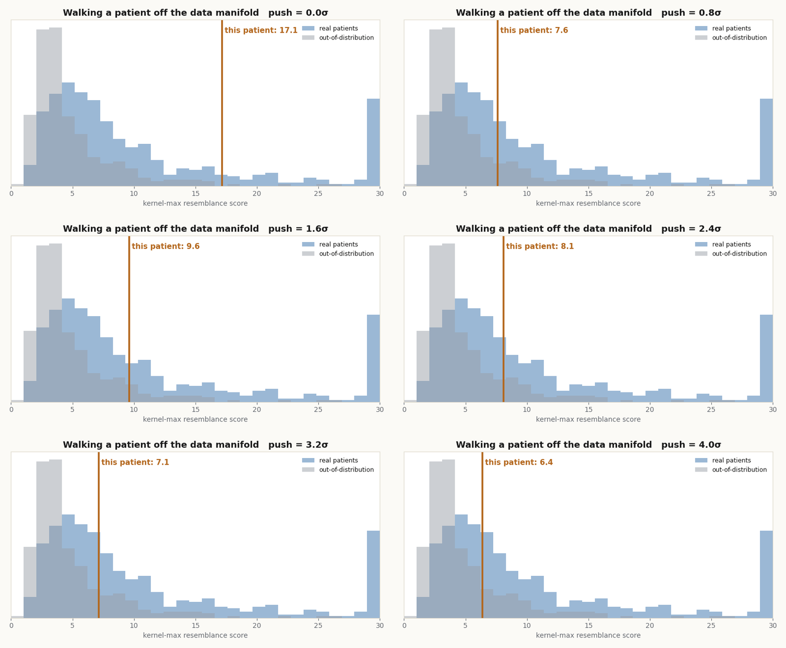
A bounded kernel gives an out-of-distribution score for free: the largest activation a patient produces is a resemblance meter. Strangers score low.
kmax = phi.max(1)                                     # kernel-max resemblance per patient
# real patients: median 7.1; synthetic out-of-distribution patients: median 3.7
Walk a real patient off the data manifold and watch the meter fall into the region where the model should decline to answer.
scripts/yat_deepsurv.py.Calibration comes along
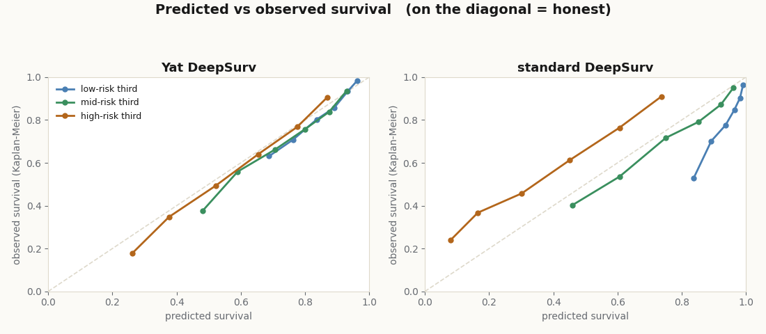
Because the Yat trunk’s log-risks are read off bounded kernels, its predicted survival tracks the observed survival closely, group by group. Bin the held-out patients into risk tertiles, and for each tertile compare the model’s mean predicted survival against the Kaplan-Meier estimate at a set of horizons: on the diagonal is honest.
scripts/yat_deepsurv.py.That is the whole white-box DeepSurv: one loss, two trunks, and a handful of array operations that turn the legible trunk’s one number into reasons, an edit, and an abstention. The explainer is where the clinical story lives.
Cite as
Bouhsine, T. (). A White-Box DeepSurv, in JAX/Flax NNX. Records of the !mmortal Data Scientist. https://tahabouhsine.com/blog/a-risk-model-that-names-its-reasons-jax-flax-nnx/
BibTeX
@misc{bouhsine2026ariskmodelthatnamesitsreasonsjaxflaxnnx,
  author       = {Bouhsine, Taha},
  title        = {A White-Box DeepSurv, in JAX/Flax NNX},
  year         = {2026},
  month        = {jul},
  howpublished = {\url{https://tahabouhsine.com/blog/a-risk-model-that-names-its-reasons-jax-flax-nnx/}},
  note         = {Blog post, Records of the !mmortal Data Scientist}
}References
- (2018). DeepSurv: Personalized Treatment Recommender System Using a Cox Proportional Hazards Deep Neural Network. BMC Medical Research Methodology 18(1), 24.arXiv:1606.00931
- (1972). Regression Models and Life-Tables. Journal of the Royal Statistical Society, Series B 34(2), 187–220.
- (1982). Evaluating the Yield of Medical Tests. JAMA 247(18), 2543–2546.
- (2012). The Genomic and Transcriptomic Architecture of 2,000 Breast Tumours (METABRIC). Nature 486, 346–352.
- (2026). A Universal Reproducing Kernel Hilbert Space from Polynomial Alignment and IMQ Distance. arXiv:2605.03262