U-Net Semantic Segmentation
Label every pixel, not just the whole image: a U-Net takes an image in and returns a same-size map of per-pixel predictions.
This guide builds directly on the encoder-decoder idea from the Autoencoder (the decoder here upsamples the very same way) and on convolutional building blocks from the Simple CNN and ResNet architecture guides (U-Net's skip connections generalize residual connections).
- What dense (per-pixel) prediction is and how it differs from classification
- How to build the U-Net encoder-decoder with a contracting and an expanding path
- Why skip connections that concatenate encoder features are the whole point
- Upsampling with
nnx.ConvTransposeback to the input resolution - Training with per-pixel sigmoid BCE and measuring quality with IoU / Dice
See the full, runnable implementation:
examples/vision/unet_segmentation.py
The Motivation
A classifier answers "what is in this image?" with a single label. Semantic segmentation answers a much harder question — "what is at every pixel?" — by producing an output map the same height and width as the input, where each pixel carries its own prediction. That is exactly what you need for medical imaging, autonomous driving, satellite analysis, and background removal.
The difficulty is a tension between two things:
- Context: to know what a pixel is, the network needs a large receptive field, which means downsampling to see the big picture.
- Localization: to know where an object's boundary lies, the network needs full-resolution detail, which downsampling throws away.
U-Net (Ronneberger et al., 2015) resolves the tension with a symmetric encoder-decoder plus skip connections. The encoder downsamples to gather context; the decoder upsamples back to full resolution; and skip connections splice the encoder's high-resolution features directly into the decoder so fine boundaries are never lost. Drawn out, the data flow makes a "U" — hence the name.
The Architecture
Each decoder stage does not just consume the layer below it — it concatenates the matching encoder features along the channel axis:
That concatenation () is the skip connection. It hands the decoder the sharp, high-resolution activations the encoder computed before pooling them away, which is what lets a U-Net trace crisp object boundaries.
The building block: a double conv
Every stage is a (Conv → GroupNorm → ReLU) × 2 block at a fixed resolution. We
use nnx.GroupNorm rather than nnx.BatchNorm so normalization is
batch-independent — convenient with nnx.jit and the small batches you'll run on
CPU. Keep channel counts divisible by num_groups.
import jax, jax.numpy as jnp
from flax import nnx

class DoubleConv(nnx.Module):
    """(Conv -> GroupNorm -> ReLU) x 2 at a fixed spatial resolution."""
    def __init__(self, in_ch, out_ch, *, num_groups=8, rngs):
        self.conv1 = nnx.Conv(in_ch, out_ch, kernel_size=(3, 3), padding='SAME', rngs=rngs)
        self.norm1 = nnx.GroupNorm(out_ch, num_groups=num_groups, rngs=rngs)
        self.conv2 = nnx.Conv(out_ch, out_ch, kernel_size=(3, 3), padding='SAME', rngs=rngs)
        self.norm2 = nnx.GroupNorm(out_ch, num_groups=num_groups, rngs=rngs)

    def __call__(self, x):
        x = nnx.relu(self.norm1(self.conv1(x)))
        x = nnx.relu(self.norm2(self.conv2(x)))
        return x
The U-Net
The encoder halves the resolution twice with nnx.max_pool; the bottleneck runs
at the coarsest scale; and the decoder upsamples with nnx.ConvTranspose,
concatenating the stored skip at each step. A final 1×1 conv projects to
per-pixel logits — one channel here, since the task is binary foreground vs.
background.
class UNet(nnx.Module):
    """A 2-level U-Net for binary semantic segmentation."""
    def __init__(self, in_channels=1, out_channels=1, base=16, *, rngs):
        # Encoder (contracting path)
        self.enc1 = DoubleConv(in_channels, base, rngs=rngs)        # full res
        self.enc2 = DoubleConv(base, base * 2, rngs=rngs)           # 1/2 res
        # Bottleneck
        self.bottleneck = DoubleConv(base * 2, base * 4, rngs=rngs)  # 1/4 res
        # Decoder (expanding path): ConvTranspose doubles resolution; the
        # following DoubleConv sees upsampled features ++ encoder skip (2x in_ch).
        self.up2 = nnx.ConvTranspose(base * 4, base * 2, kernel_size=(3, 3),
                                     strides=(2, 2), padding='SAME', rngs=rngs)
        self.dec2 = DoubleConv(base * 4, base * 2, rngs=rngs)       # concat -> base*4
        self.up1 = nnx.ConvTranspose(base * 2, base, kernel_size=(3, 3),
                                     strides=(2, 2), padding='SAME', rngs=rngs)
        self.dec1 = DoubleConv(base * 2, base, rngs=rngs)          # concat -> base*2
        # 1x1 conv -> per-pixel class logits (no activation)
        self.out_conv = nnx.Conv(base, out_channels, kernel_size=(1, 1), rngs=rngs)

    def __call__(self, x, train=False):
        # Encoder: store s1, s2 as skip sources BEFORE each downsample.
        s1 = self.enc1(x)                                          # (B,H,  W,  base)
        s2 = self.enc2(nnx.max_pool(s1, (2, 2), strides=(2, 2)))   # (B,H/2,W/2,base*2)
        b = self.bottleneck(nnx.max_pool(s2, (2, 2), strides=(2, 2)))  # (B,H/4,..,base*4)
        # Decoder: upsample, concatenate the skip, then DoubleConv.
        d2 = self.up2(b)                                           # (B,H/2,W/2,base*2)
        d2 = self.dec2(jnp.concatenate([d2, s2], axis=-1))         # skip 2
        d1 = self.up1(d2)                                          # (B,H,  W,  base)
        d1 = self.dec1(jnp.concatenate([d1, s1], axis=-1))         # skip 1
        return self.out_conv(d1)                                   # (B,H,W,out) logits
A ResNet block adds its skip (x + f(x)), which requires matching channel
counts and fuses the two signals. U-Net concatenates ([a ‖ b]), preserving
both the upsampled semantic features and the raw encoder detail as separate
channels for the next conv to mix as it sees fit. That is why the decoder's
DoubleConv takes twice the channels it outputs.
The Loss: Per-Pixel Sigmoid BCE
Binary segmentation is just binary classification repeated at every pixel. With logits and ground-truth mask over pixels ,
The shared bce_loss helper already applies optax.sigmoid_binary_cross_entropy
and sums over pixels — it works directly on 4-D (B, H, W, 1) tensors. The train
step is the textbook NNX pattern: nnx.value_and_grad with has_aux=True, then
optimizer.update.
from shared.training_utils import bce_loss

@nnx.jit
def train_step(model, optimizer, batch):
    def loss_fn(model):
        logits = model(batch['image'], train=True)   # (B, H, W, 1)
        loss = bce_loss(logits, batch['mask'])        # per-pixel sigmoid BCE
        return loss, logits
    (loss, logits), grads = nnx.value_and_grad(loss_fn, has_aux=True)(model)
    optimizer.update(model, grads)
    return loss, logits
Build the model and optimizer with explicit RNGs and the modern wrt=nnx.Param
optimizer API:
import optax
model = UNet(in_channels=1, out_channels=1, base=16, rngs=nnx.Rngs(0))
optimizer = nnx.Optimizer(model, optax.adam(1e-3), wrt=nnx.Param)
Measuring Quality: IoU and Dice
Raw BCE is hard to interpret and, because most pixels are background, a lazy all-background predictor can post a deceptively low loss. Segmentation is scored with overlap metrics between the thresholded prediction and ground truth :
def iou_dice(logits, masks, threshold=0.5, eps=1e-6):
    preds = (jax.nn.sigmoid(logits) > threshold).astype(jnp.float32)
    axes = (1, 2, 3)
    inter = jnp.sum(preds * masks, axis=axes)
    p_area, g_area = jnp.sum(preds, axis=axes), jnp.sum(masks, axis=axes)
    union = p_area + g_area - inter
    iou = jnp.mean((inter + eps) / (union + eps))
    dice = jnp.mean((2.0 * inter + eps) / (p_area + g_area + eps))
    return iou, dice
The Data: Synthetic Shapes
No downloads needed. We drop a few bright circles and squares on a dim, noisy
background; the mask is 1 wherever a shape covers a pixel. Everything is built
with jax.random, so the whole example runs offline.
def make_dataset(n=128, size=32, max_shapes=3, seed=0):
    key = jax.random.key(seed)
    k_cy, k_cx, k_r, k_shape, k_noise = jax.random.split(key, 5)
    coords = jnp.arange(size, dtype=jnp.float32)
    gy, gx = jnp.meshgrid(coords, coords, indexing='ij')       # (size, size)

    margin = 0.18 * size
    cy = jax.random.uniform(k_cy, (n, max_shapes), minval=margin, maxval=size - margin)
    cx = jax.random.uniform(k_cx, (n, max_shapes), minval=margin, maxval=size - margin)
    radius = jax.random.uniform(k_r, (n, max_shapes), minval=0.09 * size, maxval=0.20 * size)
    is_circle = jax.random.bernoulli(k_shape, 0.5, (n, max_shapes))

    dy = gy[None, None] - cy[..., None, None]                  # (n, K, H, W)
    dx = gx[None, None] - cx[..., None, None]
    r = radius[..., None, None]
    circ = (dy ** 2 + dx ** 2) <= r ** 2                       # disk
    square = (jnp.abs(dy) <= r) & (jnp.abs(dx) <= r)           # axis-aligned box
    per_shape = jnp.where(is_circle[..., None, None], circ, square)
    mask = jnp.any(per_shape, axis=1).astype(jnp.float32)      # (n, H, W) union

    noise = 0.05 * jax.random.normal(k_noise, (n, size, size))
    image = jnp.clip(0.15 + 0.70 * mask + noise, 0.0, 1.0)
    return image[..., None], mask[..., None]                   # (n, H, W, 1) each
Results / What to Expect
After a dozen epochs the U-Net segments a held-out batch of shapes almost perfectly. Each row below is one test image the model never trained on: the raw input (left), the ground-truth mask (middle), and the predicted foreground probability (right, with the thresholded boundary drawn in cyan).
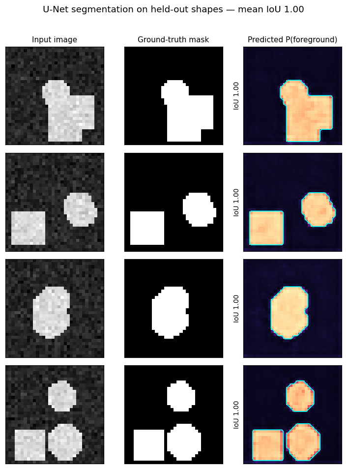
The predicted heatmaps light up exactly where the true shapes are — circles and squares alike — and the cyan decision boundary hugs the ground-truth outline (per-example IoU ≈ 1.0), demonstrating that the encoder-decoder with skip connections recovers a crisp mask at the original resolution, pixel by pixel.
The verification harness builds the model, checks the output resolution matches the input, and trains 40 steps on a fixed batch. The BCE drops sharply and the IoU climbs from near-zero (a random init predicts nearly nothing) to well above 0.9 — the shapes are cleanly segmented:
params: 130,193
input shape:  (8, 32, 32, 1)
output shape: (8, 32, 32, 1)
loss[0]=736.512  loss[-1]=172.046
IoU[0]=0.130  IoU[-1]=0.972
loss trace (every 8): [736.51, 343.26, 263.61, 215.21, 188.82]
IoU  trace (every 8): [0.13, 0.897, 0.934, 0.951, 0.961]
final IoU=0.972  Dice=0.986

ALL ASSERTS PASSED
The full script (python vision/unet_segmentation.py) trains a few epochs over a
fresh synthetic dataset and reports IoU/Dice each epoch:
  epoch  1/3 | BCE   580.57 | IoU 0.808 | Dice 0.893
  epoch  2/3 | BCE   389.29 | IoU 0.887 | Dice 0.939
  epoch  3/3 | BCE   329.37 | IoU 0.915 | Dice 0.954
Because the crucial signal is segmentation overlap rather than the raw loss value, we assert that IoU improves (and ends above 0.5), not merely that the loss goes down.
Common Pitfalls
Dropping the skip connections
❌ A plain encoder-decoder without skips produces blurry, misplaced boundaries.
✅ jnp.concatenate([upsampled, skip], axis=-1) at every decoder stage.
Channel-count mismatch after concatenation
❌ Sizing the decoder DoubleConv for the upsampled features only.
✅ Its in_ch is upsampled_ch + skip_ch (here base*2 + base*2 = base*4).
Judging the model by BCE alone ❌ Background dominates, so an all-zero mask can post a low loss. ✅ Track IoU / Dice, which reward actual overlap with the target.
Applying sigmoid before the loss
❌ Feeding probabilities into sigmoid_binary_cross_entropy double-counts it.
✅ Return raw logits from out_conv; the loss applies the sigmoid internally.
BatchNorm with tiny CPU batches
❌ nnx.BatchNorm needs the use_running_average train/eval dance and wobbles on small batches.
✅ nnx.GroupNorm normalizes per-group, batch-independently (channels divisible by num_groups).
Next steps
- Diffusion Models (DDPM) — the same encoder-decoder-with-skips U-Net becomes a time-conditioned denoiser; this guide is the "full" version its compact inline U-Net points back to.
- Vision Transformer (ViT) — an attention-based alternative backbone for dense and global image tasks.
Complete Example
examples/vision/unet_segmentation.py— a complete, CPU-verifiable U-Net: synthetic shape/mask generator, encoder-decoder with concatenating skip connections,nnx.ConvTransposeupsampling, sigmoid-BCE training step, and IoU/Dice metrics.
References
- U-Net: U-Net: Convolutional Networks for Biomedical Image Segmentation (Ronneberger, Fischer & Brox, 2015)
- Fully Convolutional Networks: Fully Convolutional Networks for Semantic Segmentation (Long, Shelhamer & Darrell, 2015)
- Group Normalization: Group Normalization (Wu & He, 2018)
- 3D U-Net: 3D U-Net: Learning Dense Volumetric Segmentation (Çiçek et al., 2016)