LSTM Time-Series Forecasting

Read the recent past, predict the near future. This guide slices a signal into sliding windows and trains an LSTM to map the last L observations to the next H values — standard supervised, multi-step forecasting in Flax NNX, all on synthetic data that needs no download.

Prerequisites

This builds directly on recurrent layers. Read recurrent networks for the nnx.RNN / nnx.LSTMCell API and the LSTM gate math, and simple training for the NNX training loop.

What you'll learn

• How to turn a raw 1-D series into (window -> horizon) supervised pairs with sliding windows
• How to build a multi-step forecaster: nnx.RNN(nnx.LSTMCell) encoder + a nnx.Linear head to H outputs
• Why forecasting uses an MSE regression loss instead of cross-entropy
• How to split in time and standardize with train statistics only so the future never leaks
• How to read the result: test_mse falling and the forecast tracking the held-out continuation

Example Code

See the full implementation: examples/sequence/time_series.py

From a series to a supervised problem

A time series is a single long vector $s_1, s_2, \dots, s_T$. To train a model with mini-batches we reframe forecasting as ordinary supervised learning using a sliding window. Pick an input length $L$ (the lookback) and a forecast length $H$ (the horizon). Every position $i$ yields one training pair:

$$\underbrace{(s_i, s_{i+1}, \dots, s_{i+L-1})}_{\text{input window } x^{(i)}} \;\longrightarrow\; \underbrace{(s_{i+L}, \dots, s_{i+L+H-1})}_{\text{target } y^{(i)}}$$

Sliding the window by one step across the series produces $N = T - L - H + 1$ overlapping examples. The model learns a single function $f_\theta: \mathbb{R}^{L} \to \mathbb{R}^{H}$ that it applies at every position — the same weight-sharing idea that makes recurrence work, now lifted to the dataset level.

This is not meta-learning

If you have seen the MAML sine-wave example, note the difference: there each sine wave is a separate task and the model adapts from a handful of shots. Here there is one series and one task; we simply cut it into many windows and do standard batched gradient descent. No inner loop, no fast weights.

The data: sum of sinusoids

Real univariate series — energy load, temperature, request rates — are dominated by a few periodic components riding on noise. We synthesize exactly that, so the example is fully offline and reproducible:

$$s_t = \sin\!\left(\tfrac{2\pi t}{24}\right) + 0.5\,\sin\!\left(\tfrac{2\pi t}{168}\right) + 0.3\,\sin\!\left(\tfrac{2\pi t}{7}\right) + 0.1\,\varepsilon_t,\qquad \varepsilon_t \sim \mathcal{N}(0,1)$$

The periodic terms make the future predictable from the past; the noise term stops the LSTM from memorizing and forces it to learn the underlying structure.

import jax
import jax.numpy as jnp


def make_series(length, *, seed=0):
    t = jnp.arange(length, dtype=jnp.float32)
    series = (
        1.0 * jnp.sin(2 * jnp.pi * t / 24.0)     # daily-like cycle
        + 0.5 * jnp.sin(2 * jnp.pi * t / 168.0)  # weekly-like cycle
        + 0.3 * jnp.sin(2 * jnp.pi * t / 7.0)    # short ripple
    )
    noise = 0.1 * jax.random.normal(jax.random.key(seed), (length,))
    return series + noise

We vmap a dynamic_slice to cut every window in one vectorized shot, adding a trailing feature axis so the shape is (N, L, 1) — exactly what nnx.RNN expects:

def make_windows(series, window, horizon):
    n = series.shape[0] - window - horizon + 1
    starts = jnp.arange(n)
    x = jax.vmap(lambda s: jax.lax.dynamic_slice(series, (s,), (window,)))(starts)
    y = jax.vmap(lambda s: jax.lax.dynamic_slice(series, (s + window,), (horizon,)))(starts)
    return x[..., None], y   # (N, window, 1), (N, horizon)

Split in time, then standardize with train stats only. We cut the series into a past (train) and a future (test) before windowing, compute the mean and std on the training region alone, and apply them everywhere. Standardizing with future statistics would leak information the model could never have at inference time.

split = int(0.8 * length)
mean = series[:split].mean()
std = series[:split].std() + 1e-6
series = (series - mean) / std

The model in Flax NNX

The forecaster is a two-line module: an LSTM encoder over the window, then a linear projection from the final hidden state to all H future values at once (a direct multi-step forecast).

from flax import nnx


class LSTMForecaster(nnx.Module):
    def __init__(self, in_features, hidden, horizon, *, rngs: nnx.Rngs):
        self.rnn = nnx.RNN(nnx.LSTMCell(in_features, hidden, rngs=rngs))
        self.head = nnx.Linear(hidden, horizon, rngs=rngs)

    def __call__(self, x):
        h = self.rnn(x)             # (B, L, in_features) -> (B, L, hidden)
        return self.head(h[:, -1])  # last step           -> (B, horizon)

nnx.RNN scans the nnx.LSTMCell across the time axis and returns every step's hidden state, (B, L, hidden). We keep the last state h[:, -1] — it has integrated the entire lookback — and the head maps it to the H-step forecast. For a univariate series in_features = 1; for multivariate input you would simply stack channels on the last axis.

The training step

Forecasting is regression, so the loss is mean squared error, not cross-entropy. Everything else is the standard NNX pattern: nnx.value_and_grad with has_aux=True to also return predictions, then optimizer.update(model, grads).

import optax
from shared.training_utils import compute_mse_loss


@nnx.jit
def train_step(model, optimizer, batch):
    def loss_fn(model):
        preds = model(batch["x"])            # (B, horizon)
        loss = compute_mse_loss(preds, batch["y"])
        return loss, preds

    (loss, preds), grads = nnx.value_and_grad(loss_fn, has_aux=True)(model)
    optimizer.update(model, grads)
    return loss, preds

Build the model and optimizer explicitly, then loop over shuffled windows:

model = LSTMForecaster(in_features=1, hidden=64, horizon=12, rngs=nnx.Rngs(0))
optimizer = nnx.Optimizer(model, optax.adam(5e-3), wrt=nnx.Param)

for epoch in range(40):
    perm = jax.random.permutation(jax.random.key(epoch), n)
    for i in range(0, n - batch_size + 1, batch_size):
        idx = perm[i:i + batch_size]
        loss, _ = train_step(model, optimizer, {"x": x_tr[idx], "y": y_tr[idx]})

Results / What to Expect

With a lookback of 48 and a horizon of 12, both the training and held-out MSE fall steadily as the LSTM locks onto the periodic structure. Because the test windows are a genuine continuation of the series, the falling test_mse is real generalization, not memorization:

$ python sequence/time_series.py
train_windows=350 test_windows=92 window=48 horizon=12 epochs=40 batch=64
epoch  0  train_mse 0.7987  test_mse 0.7126
epoch  5  train_mse 0.2200  test_mse 0.2149
epoch 10  train_mse 0.1280  test_mse 0.1634
epoch 20  train_mse 0.0723  test_mse 0.0781
epoch 30  train_mse 0.0333  test_mse 0.0470
epoch 39  train_mse 0.0255  test_mse 0.0382
held-out forecast MSE (first window): 0.0385
forecast[:4] [0.725 0.705 0.684 0.955]  truth[:4] [0.62  0.71  0.6   0.968]

The forecast on the first held-out window tracks the true continuation closely — the predicted values sit right next to the ground truth in standardized units. Environment knobs EPOCHS, BATCH, and SYNTHETIC scale the run; SYNTHETIC=0 uses a longer 2048-step series.

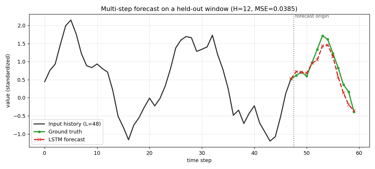
The model reads the solid black lookback window, and past the forecast-origin line its 12-step forecast (red, dashed) closely follows the true continuation (green) it never saw — direct visual evidence that the LSTM has learned the series' periodic structure rather than memorizing it.

Common Pitfalls

• ❌ Feeding a flat (B, L) window into nnx.RNN and getting a shape error. ✅ The RNN needs a feature axis: reshape to (B, L, 1) for univariate input (stack channels for multivariate).

• ❌ Standardizing the whole series (or the test split) with global mean/std. ✅ Compute statistics on the training region only and reuse them — future stats leak information you won't have at inference.

• ❌ Predicting one step and calling H steps done, or looping the model on its own noisy outputs without training for it. ✅ Emit all H values at once with a nnx.Linear(hidden, H) head (direct multi-step) so every horizon step gets its own trained weights.

• ❌ Reaching for compute_cross_entropy_loss because other sequence guides use it. ✅ Forecasting is regression over continuous values — use MSE (compute_mse_loss).

• ❌ Judging quality by raw MSE alone. ✅ Compare against a naive persistence baseline (repeat the last observed value); a useful model must beat it.

Next steps

• Word2Vec — learn dense representations from sequences instead of forecasting them.
• Simple Transformer — attention replaces the recurrent scan and forecasts every position in parallel.

Complete Example

Full runnable script with the synthetic series, sliding-window builder, time-based split, and training loop: examples/sequence/time_series.py.

References

• Hochreiter & Schmidhuber (1997), Long Short-Term Memory — Neural Computation 9(8).
• Lim & Zohren (2020), Time Series Forecasting With Deep Learning: A Survey — arXiv:2004.13408.
• Salinas et al. (2019), DeepAR: Probabilistic Forecasting with Autoregressive Recurrent Networks — arXiv:1704.04110.
• Hewamalage, Bergmeir & Bandara (2019), Recurrent Neural Networks for Time Series Forecasting: Current Status and Future Directions — arXiv:1909.00590.