Neural Ordinary Differential Equations

Instead of stacking a fixed number of layers, learn the velocity of a state and let a solver do the depth. The network becomes a continuous-time dynamical system.

Prerequisites

You should have met differential-equation losses in the PINN guide and be comfortable writing your own loop (custom training loops). Familiarity with jax.lax.scan helps but is not required.

What you'll learn

• How a Neural ODE replaces layer count with a learned vector field $f_\theta(y)$ and a numerical solver
• How to hand-write a fixed-step RK4 integrator with jax.lax.scan — no diffrax dependency
• What "discretize-then-optimize" means: backprop straight through the unrolled solver
• How to fit an entire trajectory (not point labels) with a plain MSE loss
• Why zero-initializing the dynamics keeps an untrained solver from blowing up

Example Code

See the full implementation: examples/scientific/neural_ode.py

From layers to a vector field

A residual block computes $y_{n+1} = y_n + f_\theta(y_n)$. Squint at that and it is one Euler step of a differential equation with step size $1$. A Neural ODE takes the limit seriously: instead of a discrete stack of blocks, it defines a continuous-depth state $y(t)$ whose velocity is a neural network,

$$\frac{dy}{dt} = f_\theta(t, y), \qquad y(0) = y_0 .$$

The "output" is the state at some later time $T$, obtained by integrating the field:

$$y(T) = y_0 + \int_0^T f_\theta(t, y(t))\, dt .$$

Depth is now a continuous variable, and the number of function evaluations is chosen by the solver, not baked into the architecture. Our field is autonomous ($f_\theta(y)$, no explicit $t$ dependence), which is all a spiral needs — but the solver signature keeps $t$ so you can drop in a non-autonomous field.

The task: recover a spiral

To have a ground truth we can score against, we manufacture data from a known linear ODE whose solution is a decaying spiral:

$$\frac{dy}{dt} = A y, \qquad A = \begin{bmatrix} -0.1 & -1.0 \\ 1.0 & -0.1 \end{bmatrix}, \qquad y_0 = \begin{bmatrix} 2 \\ 0 \end{bmatrix}.$$

The eigenvalues of $A$ are $-0.1 \pm i$: the imaginary part rotates (period $\approx 2\pi$), the negative real part pulls the radius inward. Integrating $A$ over $t \in [0, 8]$ gives a spiral of about $1.25$ turns. The network never sees $A$ — only the sampled trajectory it produces.

The solver: fixed-step RK4 by hand

Rather than pull in a solver library, we write the classic fourth-order Runge–Kutta step. For a step of size $h$ from $(t, y)$:

$$\begin{aligned} k_1 &= f(t, y), & k_2 &= f\!\left(t + \tfrac{h}{2},\, y + \tfrac{h}{2}k_1\right), \\ k_3 &= f\!\left(t + \tfrac{h}{2},\, y + \tfrac{h}{2}k_2\right), & k_4 &= f(t + h,\, y + h\,k_3), \\ \end{aligned}$$ $$y_{n+1} = y_n + \frac{h}{6}\left(k_1 + 2k_2 + 2k_3 + k_4\right).$$

jax.lax.scan runs the loop as a single compiled, differentiable op. Because the whole unrolled solver is just JAX primitives, reverse-mode AD flows gradients through every step — this is the discretize-then-optimize approach (differentiate the numerical scheme, as opposed to solving a separate adjoint ODE).

import jax
import jax.numpy as jnp

def rk4_step(f, y, t, dt):
    """One Runge-Kutta 4 step of dy/dt = f(t, y)."""
    k1 = f(t, y)
    k2 = f(t + dt / 2, y + dt / 2 * k1)
    k3 = f(t + dt / 2, y + dt / 2 * k2)
    k4 = f(t + dt, y + dt * k3)
    return y + dt / 6 * (k1 + 2 * k2 + 2 * k3 + k4)

def odeint_rk4(f, y0, ts):
    """Integrate dy/dt = f(t, y) over the grid `ts`, returning states (T, ...)."""
    dt = ts[1] - ts[0]

    def step(y, t):
        y_next = rk4_step(f, y, t, dt)
        return y_next, y_next

    _, ys = jax.lax.scan(step, y0, ts[:-1])
    return jnp.concatenate([y0[None], ys], axis=0)

The model

The learned dynamics is a small MLP $f_\theta : \mathbb{R}^2 \to \mathbb{R}^2$ with a smooth (gelu) activation. The NeuralODE module simply plugs that field into the solver. One important detail: we zero the output layer so the initial field is $\approx 0$. An untrained random field integrated over dozens of steps can blow up (an initial trajectory MSE in the thousands); starting from the identity flow keeps things tame.

from flax import nnx
from shared.models import MLP   # in-repo reusable MLP

class NeuralODE(nnx.Module):
    """Continuous-depth model: an MLP dynamics f_theta(y) plugged into RK4."""

    def __init__(self, hidden: int = 64, *, rngs: nnx.Rngs):
        self.func = MLP(
            in_features=2, hidden_features=hidden, out_features=2,
            n_layers=3, rngs=rngs, activation="gelu",
        )
        # Start from the identity flow: zero the final layer so f_theta(y) ~ 0.
        self.func.output.kernel[...] = jnp.zeros_like(self.func.output.kernel[...])
        self.func.output.bias[...] = jnp.zeros_like(self.func.output.bias[...])

    def dynamics(self, t, y):
        """Learned vector field; autonomous, so the time input is unused."""
        return self.func(y)

    def __call__(self, y0, ts):
        """Integrate the learned field from y0 over ts -> trajectory (T, 2)."""
        return odeint_rk4(self.dynamics, y0, ts)

Fitting a trajectory

There are no (x, y) labels here — the supervision is an entire trajectory. We integrate the learned field from the same $y_0$ over the same time grid and minimize the mean-squared error against the observed spiral:

$$\mathcal{L}(\theta) = \frac{1}{T}\sum_{i=1}^{T} \big\lVert \hat y_\theta(t_i) - y^{\text{true}}(t_i) \big\rVert^2 .$$

The train step is the standard NNX pattern; the only twist is that batch carries the initial state, the time grid, and the target trajectory:

import optax
from shared.training_utils import compute_mse_loss

@nnx.jit
def train_step(model, optimizer, batch):
    y0, ts, target = batch

    def loss_fn(model):
        pred = model(y0, ts)                 # (T, 2)
        loss = compute_mse_loss(pred, target)
        return loss, pred

    (loss, pred), grads = nnx.value_and_grad(loss_fn, has_aux=True)(model)
    optimizer.update(model, grads)
    return loss, pred

The driver builds the ground-truth spiral once (by integrating the known $A$ with the same RK4 routine) and then runs Adam:

# The known linear ODE that generates the ground-truth spiral.
A_true = jnp.array([[-0.1, -1.0], [1.0, -0.1]])
def true_dynamics(t, y):
    return y @ A_true.T                          # dy/dt = A y

y0 = jnp.array([2.0, 0.0])
rngs = nnx.Rngs(0)
model = NeuralODE(hidden=64, rngs=rngs)
optimizer = nnx.Optimizer(model, optax.adam(5e-3), wrt=nnx.Param)

ts = jnp.linspace(0.0, 8.0, 80)
true_traj = odeint_rk4(true_dynamics, y0, ts)   # (80, 2) — the observations
batch = (y0, ts, true_traj)

for step in range(1000):
    loss, _ = train_step(model, optimizer, batch)

Results / What to expect

On CPU this runs in a few seconds. Thanks to the zero-init, the trajectory MSE starts around $2.7$ (the network holds still at $y_0$) and falls by roughly six orders of magnitude — with small Adam wiggles — as the field learns to curl into a spiral:

$ python scientific/neural_ode.py
Fitting dy/dt = f_theta(y) to a spiral on t in [0, 8.0]
steps=1000  points=80

step     0 | trajectory MSE 2.7076e+00
step   100 | trajectory MSE 7.9094e-04
step   200 | trajectory MSE 1.9140e-04
step   300 | trajectory MSE 7.7715e-05
step   400 | trajectory MSE 3.5219e-05
step   500 | trajectory MSE 2.0120e-05
step   600 | trajectory MSE 1.0311e-05
step   700 | trajectory MSE 7.3010e-05
step   800 | trajectory MSE 4.4379e-06
step   900 | trajectory MSE 2.9155e-06
step   999 | trajectory MSE 2.3754e-05

final trajectory MSE = 4.6880e-06
endpoint error |y_pred(T) - y_true(T)| = 0.0055

The learned field reproduces the spiral to a final MSE of about $5\times10^{-6}$, and the predicted endpoint lands within $\sim 0.006$ of the true one — all without ever being told the generating matrix $A$.

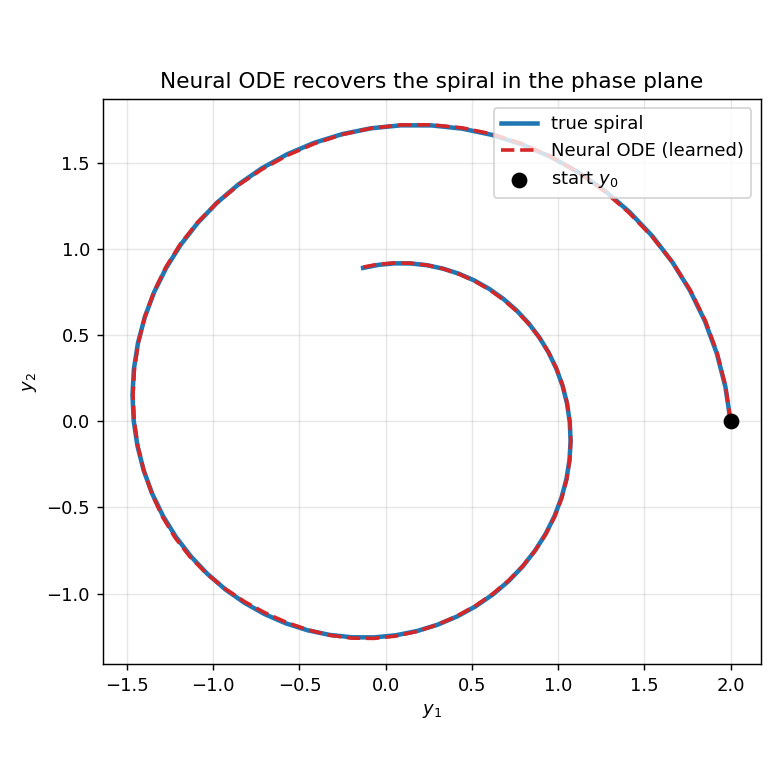
In the $y_1$–$y_2$ phase plane the learned trajectory (dashed red) sits directly on top of the true spiral (solid blue) as both curl inward from the start point — visual proof that the MLP has recovered the hidden dynamics $dy/dt = Ay$ from the trajectory alone.

Scale the run with environment variables: EPOCHS (optimization steps) and BATCH (number of points sampled along the trajectory).

Common Pitfalls

• ❌ A random, un-scaled initial field. Integrating an untrained network over dozens of RK4 steps can make the state explode (initial MSE in the thousands, sometimes NaN). ✅ Zero the last layer of the dynamics so $f_\theta(y)\approx 0$ at init — start from the identity flow, as above.

• ❌ A for loop in Python over time steps. Unrolling by hand is slow to trace and won't fuse. ✅ Use jax.lax.scan; it compiles the whole integration into one differentiable op.

• ❌ Mismatched time grids. Training on a fine grid but evaluating on a coarse one (or vice-versa) changes the discretization error and the effective dynamics. ✅ Integrate predictions and targets on the same ts; treat the grid as part of the model.

• ❌ A step size too large for the dynamics. Fixed-step RK4 is only stable when $h$ resolves the fastest timescale; too big a dt diverges regardless of the network. ✅ Pick enough points that $h$ is well below the oscillation period (here $\approx 2\pi$), or switch to an adaptive solver for stiff fields.

• ❌ A plain Python list of submodules. self.layers = [ ... ] breaks the pytree machinery on Flax 0.12. ✅ Wrap submodule lists in nnx.List([ ... ]) (and dicts in nnx.Dict).

Next steps

• Graph Neural Networks — the other frontier of structured, physics-flavored models in this track.
• Meta-learning — where differentiating through an inner optimization loop echoes differentiating through this solver.

Complete Example

examples/scientific/neural_ode.py — a self-contained Neural ODE that fits a 2D spiral with a hand-written RK4 solver and reports the final trajectory MSE and endpoint error.

References

• Chen, Rubanova, Bettencourt, Duvenaud. Neural Ordinary Differential Equations. arXiv:1806.07366
• Kidger. On Neural Differential Equations. arXiv:2202.02435
• Dupont, Doucet, Teh. Augmented Neural ODEs. arXiv:1904.01681
• Rubanova, Chen, Duvenaud. Latent ODEs for Irregularly-Sampled Time Series. arXiv:1907.03907