Variational Autoencoder (VAE)

Turn an autoencoder's bottleneck into a probability distribution you can sample from, and generate brand-new digits.

Prerequisites

Autoencoders — the encoder/decoder and nnx.ConvTranspose upsampling this guide reuses.
Understanding State & RNGs — why NNX makes randomness explicit.

What you'll learn

Why a plain autoencoder's latent space can't be sampled, and how a VAE fixes it.
The ELBO objective: a reconstruction term plus a KL regularizer, in closed form.
The reparameterization trick that lets gradients flow through a random sample.
How Flax NNX's explicit RNG streams (params vs. noise) cleanly separate weight init from latent sampling.
Reusing shared ConvEncoder / ConvDecoder bodies for the encoder and decoder.

Example Code

The complete, runnable script for this guide lives at examples/generative/vae.py.

From autoencoder to VAE

A plain autoencoder maps each image to a single point in latent space. That's great for reconstruction, but the latent space is full of holes: pick a random point and the decoder produces garbage, because nothing forced nearby points to be meaningful.

A variational autoencoder fixes this by making the encoder output a distribution instead of a point — a Gaussian $q(z \mid x) = \mathcal{N}(\mu, \operatorname{diag}(\sigma^2))$ — and by pulling every one of those Gaussians toward a shared prior $p(z) = \mathcal{N}(0, I)$ . Once training packs the latent space against that prior, you can sample $z \sim \mathcal{N}(0, I)$ and decode it into a realistic new digit.

The math: the ELBO

We want to maximize the likelihood $p(x)$ , but the marginal is intractable. Instead we maximize a tractable lower bound, the evidence lower bound (ELBO):

\mathcal{L} = \mathbb{E}_{q(z|x)}\big[\log p(x|z)\big] - D_{KL}\big(q(z|x)\,\|\,p(z)\big)

Two forces balance here:

The reconstruction term $\mathbb{E}_{q(z|x)}[\log p(x|z)]$ wants the decoder to rebuild $x$ from its latent code. For binary/greyscale pixels we model $p(x|z)$ as independent Bernoullis, so $-\log p(x|z)$ is the sigmoid binary cross-entropy between the decoder logits and the input.
The KL term $D_{KL}(q(z|x)\|p(z))$ pulls each encoded Gaussian toward the prior. For two Gaussians it has a closed form (no sampling needed):

D_{KL}\big(\mathcal{N}(\mu, \sigma^2)\,\|\,\mathcal{N}(0, I)\big) = -\tfrac{1}{2} \sum_{j} \Big(1 + \log \sigma_j^2 - \mu_j^2 - \sigma_j^2\Big)

We minimize the negative ELBO: loss = recon + kl.

The reparameterization trick

To train with gradient descent we need to backprop through the sampling step $z \sim q(z|x)$ — but sampling is not differentiable. The trick is to move the randomness outside the parameters:

z = \mu + \sigma \odot \epsilon, \qquad \epsilon \sim \mathcal{N}(0, I)

Now $\mu$ and $\sigma$ are deterministic functions of the weights, $\epsilon$ is an external noise source, and gradients flow cleanly into the encoder. In practice we predict $\log \sigma^2$ (logvar) for numerical stability and recover $\sigma = \exp(\tfrac{1}{2}\log \sigma^2)$ .

Why NNX explicit RNG streams matter

The VAE needs randomness in two unrelated places: initializing weights, and drawing $\epsilon$ every forward pass. If they shared one stream, changing the model size would shift your sampling noise, and vice versa — a debugging nightmare. Flax NNX makes each stream a named, independent generator:

rngs = nnx.Rngs(params=0, noise=1)   # weight init vs. latent sampling

Layers pull their init keys from the params stream, while our __call__ pulls fresh noise from self.rngs.noise(). The RNG state lives inside the model, so it is tracked correctly under nnx.jit and advances on every call.

Building the model

Encoder: two heads for μ and log σ²

The encoder reuses the shared ConvEncoder body — two stride-2 conv blocks that take a (B, 28, 28, 1) image down to (B, 7, 7, 32) — then flattens and splits into a mu head and a logvar head.

from flax import nnx
from shared.models import ConvEncoder, ConvDecoder

class Encoder(nnx.Module):
    def __init__(self, latent_dim: int, base: int = 16, *, rngs: nnx.Rngs):
        self.body = ConvEncoder(1, base, rngs=rngs)   # (B,28,28,1) -> (B,7,7,base*2)
        feat = base * 2 * 7 * 7                        # 32 * 7 * 7 = 1568
        self.mu = nnx.Linear(feat, latent_dim, rngs=rngs)
        self.logvar = nnx.Linear(feat, latent_dim, rngs=rngs)

    def __call__(self, x):
        h = self.body(x)
        h = h.reshape(h.shape[0], -1)                  # flatten
        return self.mu(h), self.logvar(h)

VAE: reparameterize and decode

The decoder is the shared ConvDecoder, which upsamples a latent vector back to (B, 28, 28, 1) logits. The VAE module ties encoder, sampling, and decoder together, and keeps a sample() helper for pure generation.

import jax
import jax.numpy as jnp

class VAE(nnx.Module):
    def __init__(self, latent_dim: int = 16, base: int = 16, *, rngs: nnx.Rngs):
        self.latent_dim = latent_dim
        self.encoder = Encoder(latent_dim, base, rngs=rngs)
        self.decoder = ConvDecoder(latent_dim, base, 1, rngs=rngs)  # -> logits
        self.rngs = rngs

    def __call__(self, x):
        mu, logvar = self.encoder(x)
        std = jnp.exp(0.5 * logvar)
        eps = jax.random.normal(self.rngs.noise(), mu.shape)  # external noise
        z = mu + std * eps                                    # reparameterization
        return self.decoder(z), mu, logvar

    def sample(self, n: int, seed: int = 0):
        z = jax.random.normal(jax.random.key(seed), (n, self.latent_dim))
        return nnx.sigmoid(self.decoder(z))                   # logits -> [0, 1]

Note the decoder returns logits in __call__ (so the loss can use numerically stable sigmoid-BCE) but sample() applies nnx.sigmoid to produce viewable pixels in $[0, 1]$ .

The loss and train step

The loss returns the negative ELBO plus its two components as auxiliary data. We reuse the shared bce_loss (summed sigmoid BCE per image) and kl_divergence (the closed-form Gaussian KL above).

from shared.training_utils import bce_loss, kl_divergence

def vae_loss(model, x):
    logits, mu, logvar = model(x)
    recon = bce_loss(logits, x)        # -E_q[log p(x|z)]
    kl = kl_divergence(mu, logvar)     # D_KL(q(z|x) || N(0, I))
    return recon + kl, (recon, kl)

The train step follows the standard NNX pattern — nnx.value_and_grad with has_aux=True, then optimizer.update(model, grads):

@nnx.jit
def train_step(model, optimizer, batch):
    def loss_fn(model):
        return vae_loss(model, batch)

    (loss, (recon, kl)), grads = nnx.value_and_grad(loss_fn, has_aux=True)(model)
    optimizer.update(model, grads)
    return loss, (recon, kl)

Wire it together with two RNG streams and Adam:

import optax

rngs = nnx.Rngs(params=0, noise=1)
model = VAE(latent_dim=16, rngs=rngs)
optimizer = nnx.Optimizer(model, optax.adam(1e-3), wrt=nnx.Param)

Results / What to expect

The script defaults to tiny synthetic data (smooth Gaussian blobs, no downloads) so it runs offline on CPU in seconds. You should see the negative ELBO fall steadily as reconstruction improves while the KL term settles:

$ python generative/vae.py
epoch 1/3  ELBO loss 545.47  (recon 531.13  kl 0.51)
epoch 2/3  ELBO loss 511.34  (recon 492.09  kl 1.00)
epoch 3/3  ELBO loss 450.06  (recon 392.50  kl 20.26)
generated samples: (8, 28, 28, 1)

Early on the KL term sits near zero (the encoder collapses to the prior while it learns to reconstruct); as training continues the latent code starts carrying information and the KL grows — exactly the reconstruction-vs-regularization balance the ELBO trades off.

On real MNIST (SYNTHETIC=0, 80 epochs), decoding the posterior mean back to pixels recovers the input through the probabilistic latent:

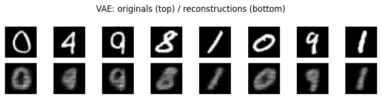
VAE reconstructions: original MNIST digits (top row) and reconstructions decoded from the posterior mean (bottom row)

Top: real inputs. Bottom: each digit encoded to (mu, logvar), then decoded from mu. The reconstructions are soft — a VAE trades sharpness for a smooth, samplable latent space — but clearly the same digits.

Avoiding posterior collapse

If reconstructions come out as identical grey blobs, the KL term has overpowered reconstruction and the decoder is ignoring the latent (posterior collapse). The fix is a β-VAE: down-weight the KL with loss = recon + β·kl for β < 1 (this script exposes a BETA env knob; the image above used BETA=0.15).

Set SYNTHETIC=0 to train on real MNIST via tfds, and tune EPOCHS / BATCH / BETA via environment variables. As training continues the KL term grows as the latent space organizes toward the prior — after which model.sample(n, seed) yields novel digits sampled from that latent.

Common Pitfalls

❌ Predicting $\sigma$ directly and taking its log (can go negative → NaN). ✅ Predict logvar and use std = jnp.exp(0.5 * logvar); the exp keeps $\sigma > 0$ .
❌ Sampling with z = jax.random.normal(...) inside loss_fn from a key you reuse every step (frozen or duplicated noise). ✅ Pull fresh noise from an NNX stream, self.rngs.noise(), so each call advances the RNG state and nnx.jit tracks it.
❌ Applying sigmoid before the loss and then using BCE (double sigmoid, unstable). ✅ Keep the decoder's __call__ output as logits and feed them to sigmoid-BCE; only apply nnx.sigmoid when you want images to look at.
❌ Dropping the KL term (or averaging BCE over pixels while summing KL). The two terms end up on wildly different scales and the model ignores the prior. ✅ Sum BCE over pixels and sum KL over latent dims, then average both over the batch — as the shared bce_loss and kl_divergence do.
❌ Sharing one RNG stream for weights and sampling (nnx.Rngs(0)), so resizing the model silently changes your noise. ✅ Use named streams: nnx.Rngs(params=0, noise=1).

Next steps

Generative Adversarial Networks (GAN) — learn the data density implicitly with an adversarial game instead of an explicit ELBO.
Diffusion Models (DDPM) — generate by iteratively denoising, trading one latent draw for many refinement steps.

Complete Example

The full, verified script is at examples/generative/vae.py — a CPU-friendly VAE with synthetic-data defaults, ELBO training loop, and a sample() generator.

References

Kingma & Welling, Auto-Encoding Variational Bayes (2013). arXiv:1312.6114
Rezende, Mohamed & Wierstra, Stochastic Backpropagation and Approximate Inference in Deep Generative Models (2014). arXiv:1401.4082
Doersch, Tutorial on Variational Autoencoders (2016). arXiv:1606.05908
Higgins et al., β-VAE: Learning Basic Visual Concepts with a Constrained Variational Framework (2017). OpenReview

From autoencoder to VAE​

The math: the ELBO​

The reparameterization trick​

Why NNX explicit RNG streams matter​

Building the model​

Encoder: two heads for μ and log σ²​

VAE: reparameterize and decode​

The loss and train step​

Results / What to expect​

Common Pitfalls​

Next steps​

Complete Example​

References​