Q and K Projections in JAX/Flax NNX

The explainer argued that $Q$ and $K$ projections turn a dot product into a learned, low-rank, role-aware bilinear form $s_{ij}=x_i^\top W_Q W_K^\top x_j$. This is the implementation companion: the Flax NNX attention module, the bilinear form pulled back out of it, its symmetric/antisymmetric split, a toy induction head, RoPE, and the two facts about the factorization you can check with a single assert: the rank budget and the gauge freedom.

The whole post is plain JAX and Flax NNX. Nothing here needs a GPU; the shapes are tiny on purpose, because the point is to see the bilinear form, not to benchmark it.

Scaled dot-product attention, with the roles exposed#

A head makes two views of each token and compares them. In NNX that is two nnx.Linear layers for $Q$ and $K$, one for $V$, one for the output, and a scaled dot product in between.

import jax
import jax.numpy as jnp
from flax import nnx


class Attention(nnx.Module):
    def __init__(self, d_model: int, n_heads: int, *, rngs: nnx.Rngs):
        assert d_model % n_heads == 0
        self.n_heads = n_heads
        self.d_head = d_model // n_heads
        # No bias on q/k: the bilinear form B = W_Q W_Kᵀ is what we want to study.
        self.q = nnx.Linear(d_model, d_model, use_bias=False, rngs=rngs)
        self.k = nnx.Linear(d_model, d_model, use_bias=False, rngs=rngs)
        self.v = nnx.Linear(d_model, d_model, rngs=rngs)
        self.o = nnx.Linear(d_model, d_model, rngs=rngs)

    def split(self, x):  # [b, t, d_model] -> [b, h, t, d_head]
        b, t, _ = x.shape
        return x.reshape(b, t, self.n_heads, self.d_head).transpose(0, 2, 1, 3)

    def __call__(self, x, *, causal: bool = True):
        q, k, v = self.split(self.q(x)), self.split(self.k(x)), self.split(self.v(x))
        scale = 1.0 / jnp.sqrt(self.d_head)            # 1/sqrt(d_k), not 1/d_k
        scores = jnp.einsum("bhid,bhjd->bhij", q, k) * scale
        if causal:
            t = x.shape[1]
            mask = jnp.tril(jnp.ones((t, t), dtype=bool))
            scores = jnp.where(mask, scores, -jnp.inf)
        attn = jax.nn.softmax(scores, axis=-1)
        y = jnp.einsum("bhij,bhjd->bhid", attn, v).transpose(0, 2, 1, 3)
        return self.o(y.reshape(x.shape))

The one number worth pausing on is scale. The entries of $x_i^\top B x_j$ grow with the head dimension, so the score is divided by $\sqrt{d_k}$ (not $d_k$) to keep the softmax out of its saturated region at initialization. Get this wrong and every head collapses onto a single token before training starts.

The bilinear form is hiding in the weights#

nnx.Linear computes $y = xK$ with kernel $K$ of shape [in, out], so the query of token $i$ is $q_i = W_Q^\top x_i$ where $W_Q$ is the kernel. The per-head score is therefore

and $B_h$ is a real matrix you can read straight out of the module.

def head_bilinear(model: Attention, h: int) -> jax.Array:
    """B_h = W_Q^(h) W_K^(h)ᵀ  in [d_model, d_model]."""
    dh = model.d_head
    Wq = model.q.kernel.value[:, h * dh:(h + 1) * dh]   # [d_model, d_head]
    Wk = model.k.kernel.value[:, h * dh:(h + 1) * dh]   # [d_model, d_head]
    return Wq @ Wk.T


model = Attention(d_model=32, n_heads=4, rngs=nnx.Rngs(0))
B = head_bilinear(model, h=0)        # [32, 32]

Two tokens score against each other through B, and the score is directed: x_i @ B @ x_j need not equal x_j @ B @ x_i.

key = jax.random.key(1)
xi, xj = jax.random.normal(key, (2, 32))
print(xi @ B @ xj)   # what i asks of j
print(xj @ B @ xi)   # what j asks of i: a different number

Splitting B into metric and direction#

Every matrix is a symmetric part plus an antisymmetric part, $B = S + A$. The symmetric part is a signed metric; the antisymmetric part is pure directedness, and it is the only source of the asymmetry above.

S = 0.5 * (B + B.T)        # symmetric: the metric
A = 0.5 * (B - B.T)        # antisymmetric: the directedness

xs = jax.random.normal(jax.random.key(2), (16, 32))
quad_B = jnp.einsum("id,de,ie->i", xs, B, xs)   # x_i^T B x_i
quad_S = jnp.einsum("id,de,ie->i", xs, S, xs)   # x_i^T S x_i
print(jnp.allclose(quad_B, quad_S, atol=1e-5))  # True

The allclose is the whole point of the symmetric/antisymmetric section in the explainer: $x^\top B x = x^\top S x$, because $A$ vanishes on the diagonal. A head’s directedness is invisible if you only score tokens against themselves; it lives entirely off-diagonal.

A shared projection (one matrix for both sides) can only produce $W W^\top$, which is symmetric and positive semidefinite. Separate $Q$ and $K$ buy two things at once: the antisymmetric $A$, and a symmetric part $S$ that is free to be indefinite. You can check the indefiniteness directly:

eigs = jnp.linalg.eigvalsh(S)
print(eigs.min(), eigs.max())   # straddles zero: S is indefinite, not a PSD metric

A toy induction head#

The cleanest directed relation is the induction head: the query reads the current token’s identity, the key reads each position’s previous token, so position $i$ attends to positions whose predecessor matches token $i$, and copies what came next.

vocab = ["a", "b", "c"]
seq = ["a", "b", "c", "a", "b", "c", "a", "b"]
idx = jnp.array([vocab.index(t) for t in seq])
E = jnp.eye(len(vocab))                 # one-hot identities

q = E[idx]                              # query = current-token identity
k = jnp.concatenate([jnp.zeros((1, len(vocab))), E[idx[:-1]]])  # key = previous token

scores = q @ k.T                        # [n, n]: 1 where tok_i == tok_{j-1}
n = len(seq)
causal = jnp.tril(jnp.ones((n, n), bool), k=-1) & (jnp.arange(n)[None, :] >= 1)
scores = jnp.where(causal, scores, -jnp.inf)
attn = jax.nn.softmax(scores / 0.1, axis=-1)

pred = attn @ E[idx]                    # copy the attended token
print(vocab[int(pred[-1].argmax())])   # -> "c": after the latest "b", predict "c"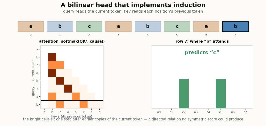

In a real model q and k are not one-hot embeddings but the outputs of W_Q and W_K; the induction circuit is just a particular $B$ that pairs current-token query features against previous-token key features. The asymmetry (“ask for my identity, answer with my predecessor”) is exactly what a non-symmetric $B$ allows and a shared projection forbids.

Position lives inside the bilinear form: RoPE#

Rotary embeddings rotate $q$ and $k$ by their positions, so the score depends only on the relative offset. The implementation is a rotate_half and a pair of cos/sin tables.

def rotate_half(x):
    x1, x2 = x[..., ::2], x[..., 1::2]
    return jnp.stack([-x2, x1], axis=-1).reshape(x.shape)


def rope(x, positions, base=10000.0):
    """x: [..., t, d_head] (d_head even); positions: [t]."""
    d = x.shape[-1]
    inv_freq = base ** (-jnp.arange(0, d, 2) / d)          # [d/2]
    ang = positions[:, None] * inv_freq[None, :]           # [t, d/2]
    cos = jnp.repeat(jnp.cos(ang), 2, axis=-1)
    sin = jnp.repeat(jnp.sin(ang), 2, axis=-1)
    return x * cos + rotate_half(x) * sin

Now the score between a fixed query and key depends only on the gap between their positions:

qv = jax.random.normal(jax.random.key(3), (8,))
kv = jax.random.normal(jax.random.key(4), (8,))
pos = jnp.arange(64)

qr = rope(jnp.broadcast_to(qv, (64, 8)), pos)
kr = rope(jnp.broadcast_to(kv, (64, 8)), pos)

# score(i, j) depends only on i - j
s = jnp.einsum("id,jd->ij", qr, kr)
print(jnp.allclose(jnp.diag(s, 5), jnp.diag(s, 5)[0], atol=1e-5))  # constant along a diagonal

Position is not added to the residual stream here; it is a rotation applied inside the bilinear form, modulating the relation $B$ itself.

Two facts about the factorization#

It is rank-limited. Because $B = W_Q W_K^\top$ with $W_Q, W_K \in \mathbb{R}^{d_\text{model}\times d_k}$, the rank of $B$ is at most $d_k$. The singular spectrum shows it: exactly $d_k$ nonzero values, the rest numerical dust.

sv = jnp.linalg.svd(B, compute_uv=False)
print(int((sv > 1e-5).sum()), "nonzero singular values, d_head =", model.d_head)
# parameters: 2*d_model*d_k  vs a full B's d_model**2

That cap is an inductive bias: each head gets a bounded relational vocabulary, and multi-head attention works because different heads spend the budget on different relations.

Only the product is identified. The split into $Q$ and $K$ is not unique. For any invertible $M$, $(W_Q M,\, W_K M^{-\top})$ gives the same $B$ and therefore the same scores: a gauge freedom.

dh = model.d_head
Wq = model.q.kernel.value[:, :dh]
Wk = model.k.kernel.value[:, :dh]
M = jax.random.normal(jax.random.key(5), (dh, dh))

Wq2 = Wq @ M
Wk2 = Wk @ jnp.linalg.inv(M).T
print(jnp.allclose(Wq @ Wk.T, Wq2 @ Wk2.T, atol=1e-4))  # True: same bilinear form

So an individual query coordinate has no canonical meaning; what is identified is the relation $B$ and the query/key subspaces it pairs, not a basis inside them.

Training, briefly#

The head is an ordinary nnx.Module, so it drops into the standard NNX loop. With current NNX, nnx.Optimizer takes wrt=nnx.Param and update receives the model and the gradients.

import optax

model = Attention(d_model=128, n_heads=8, rngs=nnx.Rngs(0))
optimizer = nnx.Optimizer(model, optax.adamw(3e-4), wrt=nnx.Param)


@nnx.jit
def train_step(model, optimizer, batch):
    x, target = batch

    def loss_fn(model):
        return jnp.mean((model(x) - target) ** 2)

    loss, grads = nnx.value_and_grad(loss_fn)(model)
    optimizer.update(model, grads)
    return loss

Nothing about the training loop knows that $W_Q$ and $W_K$ form a bilinear relation; the gradient just flows through the scaled dot product. The structure is in the parameterization, and the parameterization is the head’s relational vocabulary.

Rendering the GIFs#

Both animations are generated with Python, JAX, and matplotlib: the computation in JAX, the drawing in matplotlib:

python scripts/render_qk_bilinear_gif.py    # B = S + A, the symmetric/antisymmetric split
python scripts/render_qk_induction_gif.py   # the induction head, swept across query positions

The first renderer forms the score matrices $x^\top S x$, $\alpha\,x^\top A x$, and $x^\top B x$ on a small token cloud and animates $\alpha$; the second runs the one-hot induction attention and steps the query pointer. Neither is a benchmark; they are visual audits of the shapes, so you can see that the directedness lives off-diagonal and that the induction stripe is exactly one step below the matched positions.

What this leaves out#

A production attention layer would add dropout, KV caching for decoding, head-wise mixed precision, and a fused attention kernel (so the $N\times N$ scores never leave fast memory). It would also usually apply RoPE per-head inside __call__ rather than as the standalone function above. None of that changes the object this post is about: a learned, low-rank, role-asymmetric bilinear form, factored into a query role and a key role, then normalized into a distribution over values.

References: Flax NNX Module API; scaled dot-product attention from Vaswani et al. (2017); the QK circuit from Elhage et al. (2021); induction heads from Olsson et al. (2022); RoPE from Su et al. (2021).

@misc{bouhsine2026qkprojectionsjaxflaxnnx,
  author       = {Bouhsine, Taha},
  title        = {Q and K Projections in JAX/Flax NNX},
  year         = {2026},
  month        = {jun},
  howpublished = {\url{https://tahabouhsine.com/blog/qk-projections-jax-flax-nnx/}},
  note         = {Blog post, Records of the !mmortal Data Scientist}
}