The Prototype Readout in JAX/Flax NNX

The explainer reframed the MLP readout $W_\text{out}\,a(x)=\sum_u a_u(x)\,r_u$ as a mixture over output prototypes, whose geometry (convex, conic, affine, or linear) is set by two constraints on the coefficients: are they nonnegative, and do they sum to one? This is the implementation companion: pull the prototypes out of an NNX Linear, measure which regime each activation lands in, and build a kernel readout that is convex by construction, with the correctness checks that the explainer’s claims rest on written as asserts.

Everything here is plain JAX and Flax NNX. The dimensions are tiny so the geometry is legible.

The columns of W_out are prototypes#

An MLP block is a detector bank w_in followed by a readout w_out. In nnx.Linear the readout kernel has shape [n_units, d_out], and row $u$ is exactly the vector $r_u$ that hidden unit $u$ writes when it fires alone.

import jax
import jax.numpy as jnp
from flax import nnx


class MLP(nnx.Module):
    def __init__(self, d_in, n_units, d_out, *, rngs: nnx.Rngs):
        self.w_in = nnx.Linear(d_in, n_units, rngs=rngs)
        self.w_out = nnx.Linear(n_units, d_out, rngs=rngs)

    def prototypes(self):
        # w_out computes y = h @ kernel, so kernel[u] = r_u (the u-th output prototype).
        return self.w_out.kernel.value          # [n_units, d_out], row u = r_u

    def __call__(self, x, act=jax.nn.relu):
        h = act(self.w_in(x))                   # coefficients a_u(x)
        return self.w_out(h)                    # sum_u a_u r_u  (+ b_out)


mlp = MLP(d_in=16, n_units=64, d_out=8, rngs=nnx.Rngs(0))
R = mlp.prototypes()                            # [64, 8]

The readout is literally a coefficient-weighted sum of those rows. Writing it by hand makes the prototype view explicit (the bias just anchors the hull):

x = jax.random.normal(jax.random.key(1), (16,))
h = jax.nn.relu(mlp.w_in(x))                    # [64]
y_manual = h @ R + mlp.w_out.bias.value         # sum_u h_u r_u + b_out
print(jnp.allclose(y_manual, mlp(x), atol=1e-5))  # True

This is the same key-value picture Geva et al. (2021) found empirically: w_in rows are keys (detectors), w_out rows are values (the messages written to the stream).

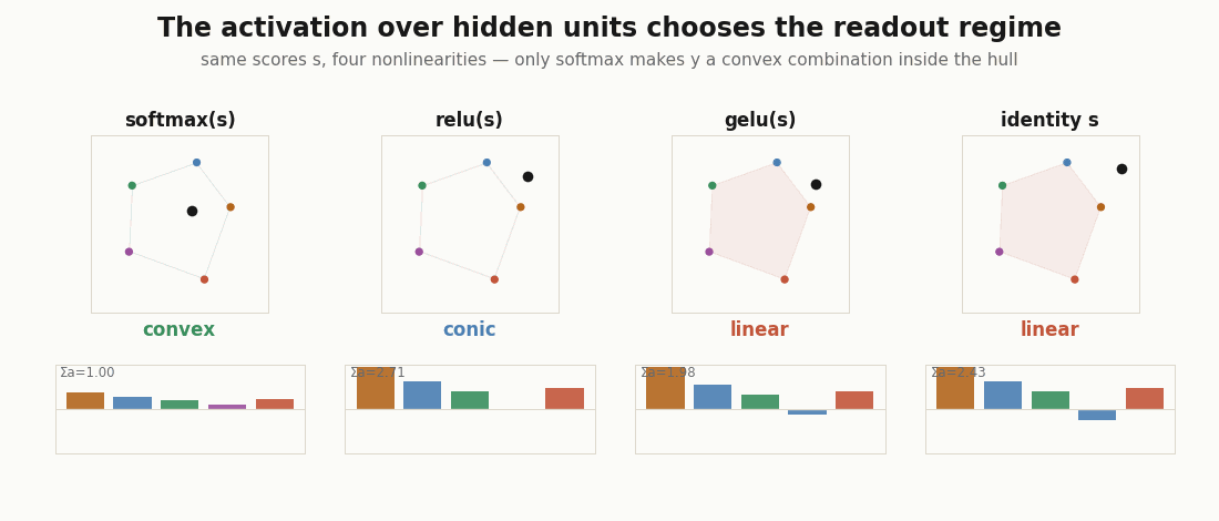
Which regime is the readout in?#

The geometry is decided by the coefficients $a(x)$, and the coefficients are decided by the activation. Two yes/no questions (nonnegative? sum to one?) sort the readout into four regimes. Here is the measurement, for the same pre-activations under different nonlinearities.

def regime(a, tol=1e-6):
    s = float(a.sum())
    nonneg = bool((a >= -tol).all())
    sum_one = abs(s - 1.0) < 1e-3
    name = ("convex" if nonneg and sum_one else
            "conic"  if nonneg else
            "affine" if sum_one else "linear")
    neg_mass = float(jnp.clip(-a, 0.0, None).sum())
    return dict(regime=name, sum=s, neg_mass=neg_mass)


s = mlp.w_in(x)                                 # raw scores over hidden units
print("softmax ", regime(jax.nn.softmax(s)))    # convex: nonneg, sums to 1
print("relu    ", regime(jax.nn.relu(s)))       # conic:  nonneg, sum free
print("gelu    ", regime(jax.nn.gelu(s)))       # linear: negative tail
print("identity", regime(s))                    # linear: signed

Only softmax gives a probability vector over hidden units, so only it makes the readout a convex combination: a point guaranteed to sit inside the convex hull of the prototypes. relu keeps the coefficients nonnegative but unnormalized (the conic regime: direction in the hull, norm as intensity). gelu and the identity admit negative coefficients, and the output can leave the hull entirely. “Unit $u$ contributed 30%” only means what it says in the first two cases.

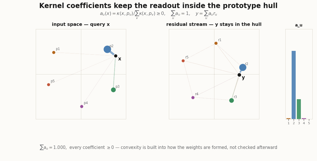
Convex by construction: a kernel readout#

The explainer’s punchline is that you do not have to hope the activation behaves. Compute the coefficients as a normalized kernel similarity to a set of input prototypes, and convexity is built in:

The requirement is that $\kappa$ be pointwise nonnegative, not that it be positive definite; these are different properties, and only nonnegativity is what convexity needs. A Flax NNX module with learnable input prototypes p, output prototypes r, and a bandwidth:

class KernelReadout(nnx.Module):
    def __init__(self, d_in, n_proto, d_out, *, rngs: nnx.Rngs):
        self.p = nnx.Param(jax.random.normal(rngs.params(), (n_proto, d_in)))   # input prototypes
        self.r = nnx.Param(jax.random.normal(rngs.params(), (n_proto, d_out)))  # output prototypes
        self.log_bw = nnx.Param(jnp.zeros(()))                                  # bandwidth

    def kernel(self, x):                          # x: [..., d_in] -> [..., n_proto]
        d2 = jnp.sum((x[..., None, :] - self.p[...]) ** 2, axis=-1)
        return jnp.exp(-d2 / (2.0 * jnp.exp(self.log_bw) ** 2))   # Gaussian: nonnegative AND PSD

    def weights(self, x):
        k = self.kernel(x)
        return k / k.sum(-1, keepdims=True)       # convex weights by construction

    def __call__(self, x):
        return self.weights(x) @ self.r[...]      # Nadaraya–Watson over learned prototypes

The convexity claims are not asserted in prose; they are assert-able:

read = KernelReadout(d_in=2, n_proto=6, d_out=2, rngs=nnx.Rngs(0))
xs = jax.random.normal(jax.random.key(2), (100, 2))
a = jax.vmap(read.weights)(xs)                    # [100, 6]

assert (a >= 0).all()                             # nonnegative
assert jnp.allclose(a.sum(-1), 1.0, atol=1e-5)    # sum to one
# every output lies inside the convex hull of the output prototypes:
ys = jax.vmap(read)(xs)
print("readout coords stay within prototype span:", float(jnp.abs(ys).max()))

Nonnegative is not the same as positive definite#

It is worth proving to yourself that the property doing the work is nonnegativity, not PSD-ness, because they are independent. The linear kernel is positive definite but takes negative values; the Gaussian and the Yat kernel are both nonnegative and positive definite.

def gram(kfn, pts):
    return jax.vmap(lambda a: jax.vmap(lambda b: kfn(a, b))(pts))(pts)

pts = jax.random.normal(jax.random.key(3), (12, 2))

linear   = lambda a, b: a @ b
gaussian = lambda a, b: jnp.exp(-0.5 * jnp.sum((a - b) ** 2))
yat      = lambda a, b: (a @ b) ** 2 / (jnp.sum((a - b) ** 2) + 1e-3)

for name, k in [("linear", linear), ("gaussian", gaussian), ("yat", yat)]:
    G = gram(k, pts)
    nonneg = bool((G >= -1e-6).all())
    psd = bool(jnp.linalg.eigvalsh(0.5 * (G + G.T)).min() >= -1e-4)
    print(f"{name:9s} nonnegative={nonneg}  PSD={psd}")
# linear   nonnegative=False PSD=True   -> would break the convex readout
# gaussian nonnegative=True  PSD=True   -> the useful corner
# yat      nonnegative=True  PSD=True   -> also the useful corner

A normalized linear kernel can produce negative “weights” and a denominator that crosses zero, meaningless as a mixture. The kernels you actually reach for sit in the nonnegative-and-PSD corner.

Choice and intensity: a gated softmax readout#

If you want the convex direction but also a learnable write intensity (the explainer’s “what to write by mixture, how much by a gate”), separate the two. This is the sparsemax/softmax-attention idea (Martins & Astudillo, 2016) applied to hidden units instead of tokens.

class GatedSoftmaxReadout(nnx.Module):
    def __init__(self, d_in, n_proto, d_out, *, rngs: nnx.Rngs):
        self.score = nnx.Linear(d_in, n_proto, rngs=rngs)
        self.gate = nnx.Linear(d_in, 1, rngs=rngs)
        self.r = nnx.Param(jax.random.normal(rngs.params(), (n_proto, d_out)))

    def __call__(self, x):
        pi = jax.nn.softmax(self.score(x), axis=-1)       # convex mixture: WHAT to write
        g = jax.nn.softplus(self.gate(x))                 # nonnegative scale: HOW MUCH
        return g * (pi @ self.r[...])

The direction pi @ r always lands in the hull; the gate scales how loudly that point is written into the residual stream.

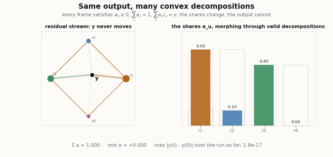
Contribution mass is not identifiable#

One caveat the explainer makes and the code makes vivid: with more hidden units than residual dimensions, the prototypes are an overcomplete dictionary, so the same output $y$ has many convex decompositions. “Unit $u$ contributed 30%” is a fact about the mechanism $a(x)$, not about $y$.

# A fixed point y inside the hull of 4 prototypes in 2-D, two EXACT convex decompositions.
R = jnp.array([[1.0, 0.0], [0.0, 1.0], [-1.0, 0.0], [0.0, -1.0]])
y = jnp.array([0.1, 0.1])

a1 = jnp.array([0.5, 0.1, 0.4, 0.0])
a2 = jnp.array([0.1, 0.5, 0.0, 0.4])

assert jnp.allclose(a1.sum(), 1.0) and jnp.allclose(a2.sum(), 1.0)   # both sum to one
assert (a1 >= 0).all() and (a2 >= 0).all()                          # both nonnegative
assert jnp.allclose(a1 @ R, y) and jnp.allclose(a2 @ R, y)          # both give exactly y
print("same y, different shares:", a1, a2)

The honest readout of a contribution number is therefore: it describes this coefficient vector, the one the layer happened to produce, not a canonical property recoverable from the output.

Training, briefly#

Each block is an nnx.Module, so they all train the same way. The kernel readout learns its input prototypes, output prototypes, and bandwidth jointly.

import optax

model = KernelReadout(d_in=16, n_proto=32, d_out=16, rngs=nnx.Rngs(0))
optimizer = nnx.Optimizer(model, optax.adamw(3e-4), wrt=nnx.Param)


@nnx.jit
def train_step(model, optimizer, batch):
    x, target = batch

    def loss_fn(model):
        return jnp.mean((jax.vmap(model)(x) - target) ** 2)

    loss, grads = nnx.value_and_grad(loss_fn)(model)
    optimizer.update(model, grads)
    return loss

The detector bank stops being an arbitrary feature extractor and becomes a similarity to named input prototypes; the readout stops being a hopeful interpretation and becomes the actual mechanism: convex by construction, not by accident.

Rendering the GIFs#

Both animations are generated with Python, JAX, and matplotlib: the computation in JAX, the drawing in matplotlib:

python scripts/render_convex_readout_gif.py          # the kernel readout tracing the hull
python scripts/render_convex_readout_regimes_gif.py  # the four activation regimes

The first renderer moves a query along a path through the input space, computes the normalized Gaussian weights and the readout each frame, and keeps a trail of $y$; the second evaluates the four nonlinearities on one oscillating score vector and places each readout against the prototype hull. They are visual audits, not benchmarks: the point is to watch convexity hold (or break) as the inputs move.

What this leaves out#

A real MLP block has a much wider hidden layer, a residual connection around it, and (in modern stacks) a gated activation like SwiGLU that pushes the coefficients further into the signed regime. The kernel readout here is a teaching variant, not a drop-in replacement; making it competitive means many more prototypes, a sharper kernel, and attention to the normalizer’s stability far from the prototype set. But the object is the same one the explainer named: a readout is a weighted sum over output prototypes, and the only question is what the weights are allowed to be.

References: Flax NNX Module API; the key-value-memory reading of feed-forward layers from Geva et al. (2021); Nadaraya–Watson regression from Nadaraya (1964); simplex-projecting activations from Martins & Astudillo (2016).

@misc{bouhsine2026convexreadoutjaxflaxnnx,
  author       = {Bouhsine, Taha},
  title        = {The Prototype Readout in JAX/Flax NNX},
  year         = {2026},
  month        = {jun},
  howpublished = {\url{https://tahabouhsine.com/blog/convex-readout-jax-flax-nnx/}},
  note         = {Blog post, Records of the !mmortal Data Scientist}
}